Highlight Rows that Meet a Certain Condition in Excel
In this tutorial I am going to cover how to highlight rows that meet a certain condition. To do this I use the Conditional Formatting tool. I will demonstrate some features of this advanced and powerful Excel tool.
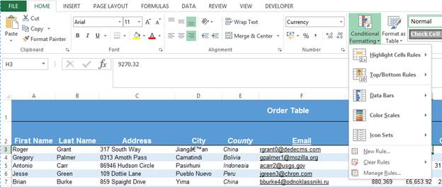
The Conditional Formatting dropdown is accessed from the Home tab:
Conditional formatting involves applying a rule to the value of a cell. If this rule evaluates true then a certain format is applied to highlight that cell. If it is false then no formatting is applied. Note that cells which do not meet the rule still keep their original formatting.
For the first example I am going to add a conditional formatting rule on the Order Total column. I am going to highlight orders which are over £5,000 in value. To do this, first I must select the Order Total column. I then navigate to the Highlight Cells Rules sub-menu of the conditional formatting menu.
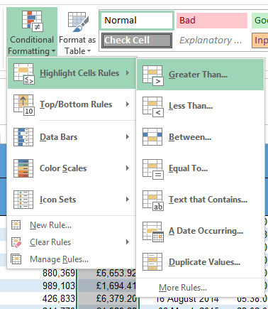
I then select the Greater than option.
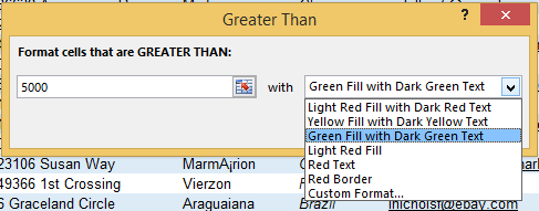
The first box is the value I want my cells to be greater than. (5000 in this case) The second box is then the formatting that is to be applied to the cells with values greater than 5000. There are a number of default options here as well as a custom formats option, should you want to be specific. For this tutorial I went with a Green Fill with Dark Green Text.
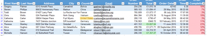
Here is the result:
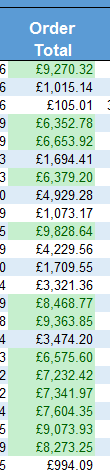
As you can see a number of cells are now highlighted as they are over the £5000. Alternatively I could have done Order Totals less than 5000 or between 1000 and 5000, or whatever I wanted. There are a number of basic rules here that you can apply to highlight cell values you are most interested in. You can even do custom rules, but this is more on the advanced side of the conditional formatting tool and will be covered in a later tutorial.
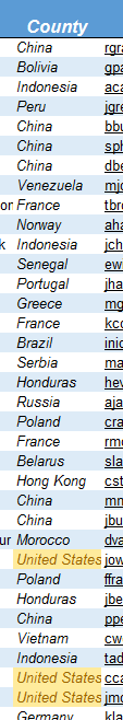
Conditional formatting doesnt just work on numerical values. You can highlight a cells value if it contains a certain text value. Although filtering may be a more useful tool for this I will demonstrate the functionality. For example I could highlight cells in the Country column where the order is from the United States.
Follow the same steps as before but, this time, select Equal to from the Highlight Cells Rules menu.
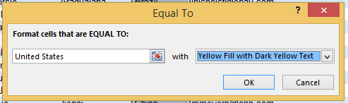
Its the same as before, just enter the required value but this time Excel is checking whether the values of the County column are equal to United States.
Another useful conditional formatting rule is to highlight the top or bottom 10, 20, 50 etc. These rules are located in the Top/Bottom Rules sub-menu of the Conditional Formatting dropdown.
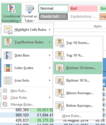
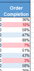
As an example I am going to highlight the bottom 10 orders by Order Completion. As before I highlight the Order Completion column and then select Bottom 10 Items from the menus. A similar menu opens up prompting for the number of top/bottom items.
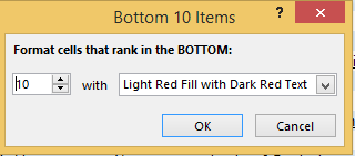
As the default options are what Im looking for I just click ok.
You can also use filtering in combination with your conditional formatting so you can easily see just the conditionally formatted rows. To do this just right-click on a cell with the conditional formatting you want to filter and select Filter by Select Cells Color.
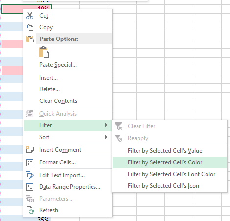
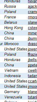
As I just highlighted the bottom 10 Order Completion cells I am going to apply a filter to see just those bottom 10 rows.
As you can see only 10 rows are displayed.
Should you want to remove a conditional formatting rule, you just select the cells you want to remove the conditional formatting from and then navigate to the Clear Rules sub-menu of the Conditional Formatting dropdown.
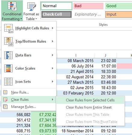
You can choose to remove the conditional formatting from the selected cells or the entire sheet should you require. For example, I am going to remove the conditional formatting on the Country column.
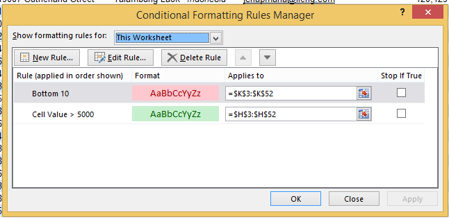
Alternatively you could add/remove rules from the Manage Rules pop-up window.
Just select it from the Conditional Formatting dropdown and then change the Show formatting rules for: box to worksheet. You then can see all the rules applied to the current worksheet. As you can see below the yellow formatting applied to the Country column is gone.
I hope this tutorial was helpful!
Dont forget to download the accompanying Excel file so you can follow along.
Question? Ask it in our Excel Forum
Excel VBA Course - From Beginner to Expert
200+ Video Lessons 50+ Hours of Instruction 200+ Excel Guides
Become a master of VBA and Macros in Excel and learn how to automate all of your tasks in Excel with this online course. (No VBA experience required.)
Tutorial: Quickly find all rows in Excel that contain a certain value and then delete those rows. ...
Tutorial: How to switch a data set in Excel so that the columns become rows and the rows become col...
Tutorial: This trick allows you to easily perform a nice visual analysis of data in Excel without m...
Macro: This macro in Excel allows you to display or show a particular comment in Excel. This will...
Tutorial: Average the results from a filtered list in Excel. This method averages only the visible ...
Tutorial: In Excel you can store values in Defined Names. Often people use a Defined Name to refe...
Subscribe for Weekly Tutorials
BONUS: subscribe now to download our Top Tutorials Ebook!
Excel VBA Course - From Beginner to Expert
200+ Video Lessons
50+ Hours of Video
200+ Excel Guides
Become a master of VBA and Macros in Excel and learn how to automate all of your tasks in Excel with this online course. (No VBA experience required.)