Average the Visible Rows in a Filtered List in Excel

Average the results from a filtered list in Excel. This method averages only the visible rows once you apply a filter.

We us the SUBTOTAL() function to do this.

Sections:

Syntax

Example - Filtered Data

Example - Exclude Manually Hidden Rows

Notes

Syntax

=SUBTOTAL(1, range_to_average)

1 tells the function to average the data.

range_to_average is the range that you want to average.

Example - Filtered Data

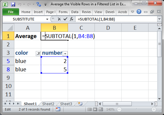
=SUBTOTAL(1,B4:B8)

This averages the data that is still visible after the filter has been applied. This works on range B4:B8.

Result:

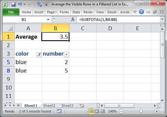
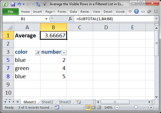
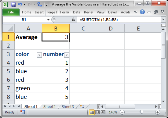
This updates when the filter is applied or changed or removed.

This only works on filtered data and not on data that was manually hidden, look to the next section to exclude manually hidden data as well.

Example - Exclude Manually Hidden Rows

Manually hidden data occurs when data is hidden via a macro or just by hand, you can see this when you select a row, right-click it, and click Hide. The above function won't work with data hidden like this unless we change the first argument.

=SUBTOTAL(101,B4:B8)

101 was 1 in the first example. Changing this to 101 makes the function ignore filtered data and also manually hidden data.

Nothing else was changed.

Notes

This function, with 1 or 101 as its first argument, simply works like a regular AVERAGE function. The only difference is that filters and hidden data are taken into account so that you can get accurate results when you are filtering and analyzing your data.

The SUBTOTAL function allows you to apply a number of regular functions to filtered data, for a full list and explanation, view our tutorial on the SUBTOTAL function in Excel.

Make sure to download the file for this tutorial so you can work with the above examples in Excel.