Sum Values that Equal 1 of Many Conditions across Multiple Columns in Excel

How to Sum values using an OR condition across multiple columns, including using OR with AND conditions. For instance, sum all the values that have red in column A or West in column B; another example is to sum the values with red in column A and West in column B or those with just West in column B.

This all sounds a bit confusing so let's get to some examples.

This tutorial assumes that you are familiar with the SUM, IF, and SUMIFS functions.

Sections:

Sum with OR Criteria

Sum with OR AND Criteria

Sum with AND Criteria (Default Method)

Get a Better Understanding of How these Formulas Work

Notes

Sum with OR Criteria

Add values that meet a condition in one column or another condition in another column.

Let's Sum the values the have red in column A or West in column B. This also includes values that have both red and West, but it does not double-count them.

=SUM(IF((A1:A6="red")+(B1:B6="west"),1,0)*C1:C6)

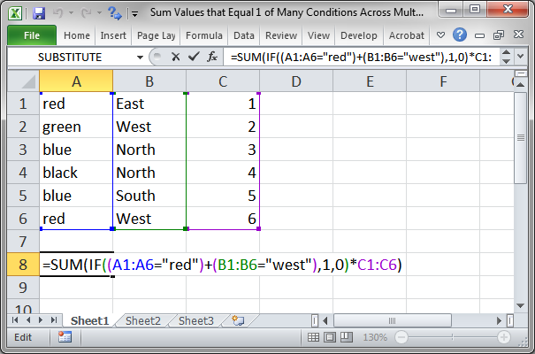
Result:

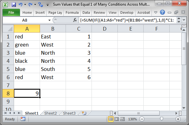
Array Formula - this is an array formula and so you must enter it into the cell using Ctrl + Shift + Enter.

The formula looks scary and confusing but there are only two parts that you have to know how to change, the criteria section and how many values across how many criteria's to check.

Criteria Section

(A1:A6="red")

This code is the syntax that you use to check for a value in a range. The range that contains the criteria goes on the left and the value that you check for goes on the right.

Enclose criteria text with double quotation marks, but if you use numbers for the criteria, you don't have to enclose it with quotation marks.

Add another Criteria Section

In the formula you will notice that the criteria sections, as described just above here, are combined using a plus sign:

(A1:A6="red")+(B1:B6="west")

To add more columns with more criteria, simply add more sections following this pattern, using a plus sign between them.

Sum with OR AND Criteria

This situation combines OR criteria with AND criteria.

Add values that have red and West values for column A and B or values that have only West in column B.

=SUM(IF((A1:A6="red")*(B1:B6="west")+(B1:B6="west"),1,0)*C1:C6)

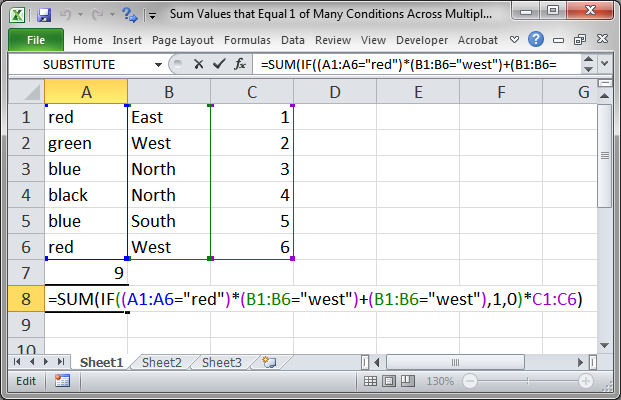
Result:

Array Formula - this is an array formula and so you must enter it into the cell using Ctrl + Shift + Enter.

Criteria Section

(A1:A6="red")

(This is the same as the last example.)

This code is the syntax that you use to check for a value in a range. The range that contains the criteria goes on the left and the value that you check for goes on the right.

Enclose criteria text with double quotation marks, but if you use numbers for the criteria, you don't have to enclose it with quotation marks.

Add another Criteria Section

In the formula you will notice that the criteria sections, as described just above here, are combined using either a plus sign or a multiplication sign:

(A1:A6="red")*(B1:B6="west")+(B1:B6="west")

The multiplication sign acts like AND and means that a value must have BOTH criteria; it must have red in column A and West in column B.

The plus sign acts like OR and means that the value will also be included if only West is in column B.

Put those two together and it reads like this: sum the values where red and West are in column A OR only West is in column B.

If you want to add more criteria sections where values must be in both columns, use the multiplication sign to join them; if you want to add more criteria sections where a value can be present in just a single column, use the plus sign to join them.

You need to download the sample file attached to this tutorial so you can work with these examples in order to get a better understanding of them.

Sum with AND Criteria (Default Method)

I included this here just so you wouldn't think that I left it out, but this method just uses the default SUMIFS function that is available in Excel 2007 and later versions.

In this example, let's sum the values that have red in column A and West in column B.

=SUMIFS(C1:C6,A1:A6,"red",B1:B6,"west")

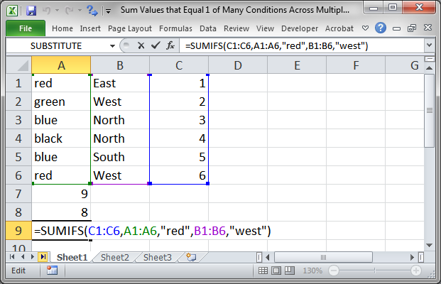
Result:

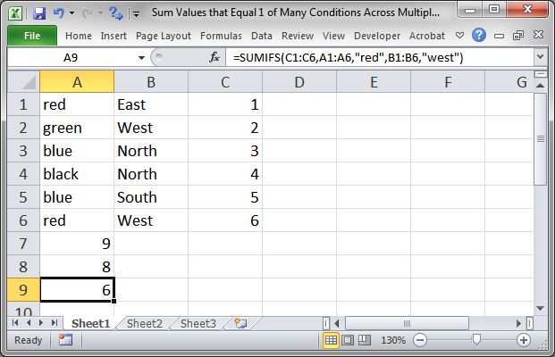
C1:C6 is the range of values that will be added together.

A1:A6 is the first criteria range.

"red" is the value that should appear in the first criteria range.

B1:B6 is the second criteria range.

"west" is the value that should appear in the second criteria range.

You follow this pattern to add as many criteria as you need, up to 127.

This is a regular formula and there isn't anything special about it or how you enter it, like there is for an array formula.

Get a Better Understanding of How these Formulas Work

The tricky stuff in this tutorial comes from using array formulas in Excel. These formulas are, almost by definition, complex and confusing and annoying, but so darn powerful.

One way to try and learn a little more about how they work is to see how Excel calculates these formulas; now this won't tell you everything, but it might help a little.

Select one of the array formulas and then go to the Formulas tab and click Evaluate Formula.

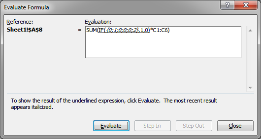
You will then be able to go through the formula to see how it works; just click the Evaluate button.

You can learn more about this feature here in our tutorial for the Evaluate Formula feature.

Notes

You cannot enter an array formula by typing curly braces around it! You will see these braces when you select an array formula and look to the Formula Bar but you cannot add or remove them yourself.

The only way to enter an array formula is by using Ctrl + Shift + Enter.

Array formulas and these examples can be really tricky and take some time to get used to, but, once you learn them, they can save you a lot of time.

Make sure you download the sample file attached to this tutorial so you can work with these examples and get a better understanding of how this works in Excel.