SUMIFS - Sum Values Based on Multiple Criteria in Excel
The SUMIFS function allows you to sum values that meet multiple criteria across multiple columns. Each value that is summed must meet each criteria that is listed in the function; this works like an AND function in that way.
Sections:
Syntax
=SUMIFS(sum_range, criteria_range1, criteria1, [criteria_range2], [criteria2],...)
| Argument | Description |
|---|---|
| Sum_range | The range of numbers that you want to sum. |
| Criteria_range1 | The range that you want to use to choose which values to sum. This must be the same size as the sum_range. |
| Criteria1 |
The criteria that you want to use to determine what to sum. This criteria is applied to the criteria_range. You must put double quotation marks around the criteria, unless you use only a number. The below example uses a number with an operator, which means it must be put within double quotation marks. To view all possible criteria operators and wildcards, go to the Criteria Operators and Wildcards sections lower in this tutorial. |
| [Criteria_range2] |
Additional criteria range. Use this to add another criteria. Max 127 criteria allowed in the SUMIFS function. This range must be the same size as the first criteria_range and the sum_range. |
| [Criteria2] | Additional criteria that applies to the additional criteria_range argument. |
[] means the argument is optional.
You can have up to 127 criteria within the SUMIFS function.
Example
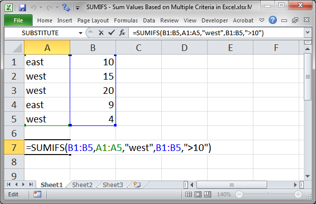
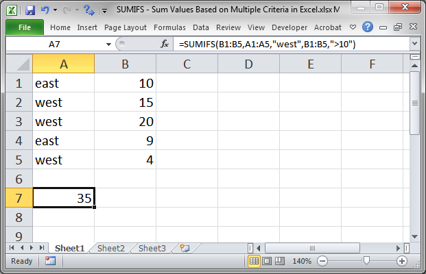
Let's sum all of the values in a list that equal west and where the values to be summed are greater than 10.
=SUMIFS(B1:B5,A1:A5,"west",B1:B5,">10")
Result:
Note: you can apply criteria to the range of values that will be summed, like I did in this example.
Function Breakdown
B1:B5 is the range of values that will be added together.
A1:A5 is the first criteria range.
"west" is the value that must appear in the first criteria range.
B1:B5 is the second criteria range.
">10" is the value that must appear in the second criteria range. I used the > (greater than) sign here and this means that only values that are greater than 10 will be added together. The next section contains more information about what you can put here.
You follow this pattern to add as many criteria as you need, up to 127.
Criteria Comparison Operators
You don't just have to check if a criterion is equal to a value; you can check if the criterion is greater than or less than a value or not equal to a value and more.
Here is a list of the comparison operators that you can use:
> Greater than. Means the values must be greater than whatever you put after this sign. This was used in the above example.
< Less than. Means the values must be less than whatever number you put after this sign.
>= Greater than or equal to. Means the values must be equal to or greater than the number that you put after this sign.
<= Less than or equal to. Means the values must be equal to or less than the number that you put after this sign.
<> Not equal to. This works for both numbers and text and says that the value must not be equal to whatever you put after this sign.
Note: it is very important that you put these signs inside of double quotation marks, even when you use them with a number (illustrated in the example above).
To learn more, check out our tutorial on comparison operators in Excel.
Wildcards
You can also use what are called wildcards in this function.
? Question mark. Matches any character. So, "Th?n" would match "Then" "Than" "Th8n" etc.
* Asterisk. Matches any number of any characters that come before, after, or in the middle of a value. So, "*hi*" would match "oh hi there" "hi there" "oh hi" etc. As you can see, you can put the asterisk before and after the value, but you can also put it only before the value if you want to match everything that comes before the value or after it to match everything that comes after it.
~ Tilde. This allows you to literally match a ? or a * character. To match a question mark, do this "~?" and to match an asterisk do this "~*" and to match a tilde with a question mark or with an asterisk do this "~~?" or this "~~*".
Wildcards can be confusing at first and they are not often used in Excel but they can be very helpful.
To learn more, check out our tutorial on wildcards in Excel.
Notes
Don't confuse the SUMIFS function with the SUMIF function. The position of the arguments is different depending on how you use the SUMIF function and so you should take note if you are switching a formula from one to the other.
Make sure that all ranges referenced in the SUMIFS function are the exact same size!
Download the sample file for this tutorial to work with the example above in Excel.
Question? Ask it in our Excel Forum
Excel VBA Course - From Beginner to Expert
200+ Video Lessons 50+ Hours of Instruction 200+ Excel Guides
Become a master of VBA and Macros in Excel and learn how to automate all of your tasks in Excel with this online course. (No VBA experience required.)
Subscribe for Weekly Tutorials
BONUS: subscribe now to download our Top Tutorials Ebook!
Excel VBA Course - From Beginner to Expert
200+ Video Lessons
50+ Hours of Video
200+ Excel Guides
Become a master of VBA and Macros in Excel and learn how to automate all of your tasks in Excel with this online course. (No VBA experience required.)