Linking Cells in Excel
In this tutorial I am going to cover how to link cells together. This is a useful feature of Excel as you can link cells in an Excel Formula instead of typing in the values each time.
Linking cells allows you to perform calculations based on the value of cells instead of typing in values. This means that you can copy Formulas over multiple cells and should the value of any linked cell change, any Formula which relies on the changed cells value will also change. Starting with a simple example of addition, I could calculate the total of a few values using the following formula:

However should I want to change any of the values in the Formula I would have to re-type it. For this reason it is better to link cells for values of a Formula/Function. To link a cell, you start by creating a Formula using the equals sign (=). You then click on the cell you want to link:

As I am looking to add together all the values in cells A1:D1, I hit the plus sign (+) in between selecting each cell. Alternatively you can type the cell references instead of selecting with the mouse.

Now that my cells are linked if I change one of their values, the cell with my addition formula (G3) will change to. This works because when a cell is linked in an Excel Formula, the calculation will be based on the values within the linked cells. If I change Cell A1 to 7 the value in cell G3 changes to 16 without me having to change the formula.

Linking cells also works within functions:

Notice how when using the Sum Function I just clicked and drag to select all the cells I require instead of selecting each cell individually. This works the same way as if I had typed =SUM(A1,B1,C1,D1) into cell I3 but is easier and quicker.
Another useful feature of linked cells is that when you move a cell which is referenced by a particular Function or Formula, the cell references within the Function/Formula will automatically update to the new cell reference where the selected cell(s) was moved to. For example, if I move cell C1 to D10:

The reference formula in cell G3 updates to D10 automatically and remains with the value 16. Its important to note here that cell references will only be automatically updated if they are directly referenced. Notice how the value in cell I3 decreases to 13. This is because I used a cell range to reference the cells. Had I moved the whole range (A1:D1) together then the cell references would have been maintained.

Linking Cells Across Different Worksheets in the Workbook
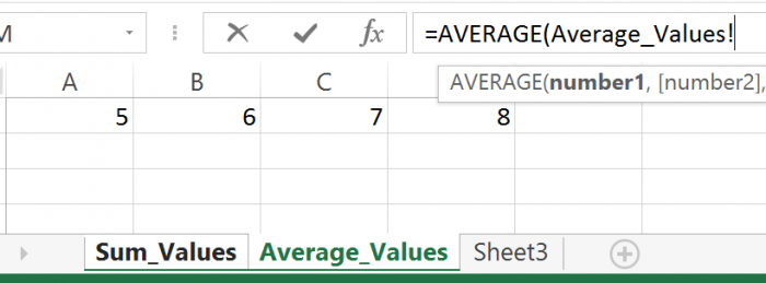
Cell referencing/linking also works across different worksheets. For the first few examples I was working from the Sum_Values sheet. I now want to use the Average Function but the values I need for this are on the Average_Values sheet. Referencing a different sheet is a similar process, just start by entering the Formula/Function you wish to use then before you select a cell, select the different sheet, then the cell.

You then select the sheet which contains the values you require:

And finally the cells you wish to use in your formula:

You then hit enter and you will be returned to the original sheet that you entered the formula on.

You can also type in the cell reference. Start with the sheet name (Average_Values) followed by an exclamation mark (!) then the cells you wish to select (A1:D1). Altogether this gives:
=Average(Average_Values!A1:D1)
Question? Ask it in our Excel Forum
Tutorial: How to use VBA/Macros to iterate through each cell in a range, either a row, a column, or ...
Tutorial: How to limit the amount that a user can enter into a range of cells in Excel. This works...
Tutorial: In this tutorial I am going to look at cell alignment / arrangement. These features allow ...
Tutorial: How to center a title across multiple cells in Excel in order to make good looking titles...
Tutorial: This Excel VBA tutorial focuses specifically on selecting ranges of cells in Excel. This...
Tutorial: How to allow only certain people to edit certain cells or ranges in Excel. This is a sec...


