Sum the Visible Rows from a Filtered List in Excel

How to SUM only the visible rows from a filtered data set in Excel.

To do this, we will use the SUBTOTAL() function.

Sections:

Syntax

Example - Filtered Data

Example - Exclude Manually Hidden Rows

Notes

Syntax

=SUBTOTAL(9, range_to_sum)

9 tells the function to perform a sum.

range_to_sum is the range that you want to sum.

Example - Filtered Data

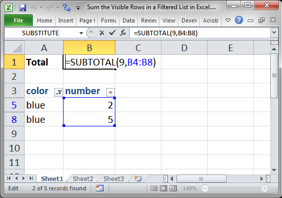
=SUBTOTAL(9,B4:B8)

This sums all visible values from a filtered list or table for the range B4:B8.

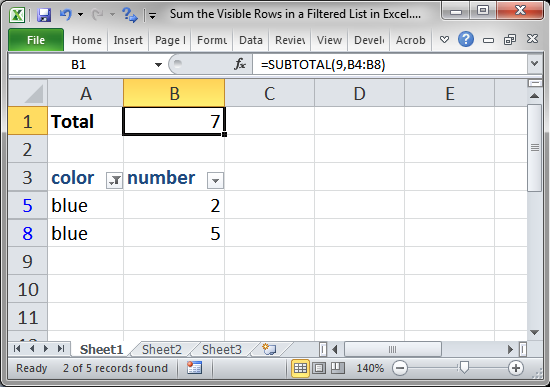
Result:

If I remove or change the filter, watch how the total will update:

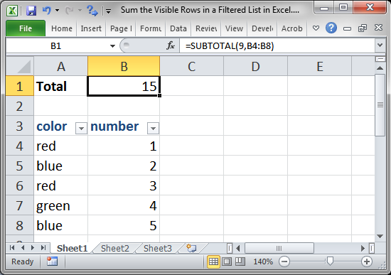
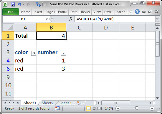
This is the beauty of this function; it works with your filtered data sets.

Example - Exclude Manually Hidden Rows

The above function only works on data that is being filtered. It does NOT work on rows that are manually hidden (right-click a row and then click Hide).

To exclude data that is also manually hidden, we change the function to this:

=SUBTOTAL(109,B4:B8)

109 this was a 9 in the first example. Changing this to 109 means that rows that are hidden via a filter and also via manually hiding the row will now not show up in the sum.

B4:B8 this is still just the range to sum.

Notes

The SUBTOTAL function allows you to apply a number of regular functions to filtered data, for a full list and explanation, view our tutorial on the SUBTOTAL function in Excel.

Make sure to download the file for this tutorial so you can work with the above examples in Excel.