Convert Column Number to Letter Using a Formula in Excel
How to get a column letter from a number in Excel using a simple formula.
This is an important thing to be able to do when working with complex formulas in Excel, especially the INDIRECT() function.
Sections:
Basic Formula - Works for A to Z
More Complex Formula - Works For All Columns
Basic Formula - Works for A to Z
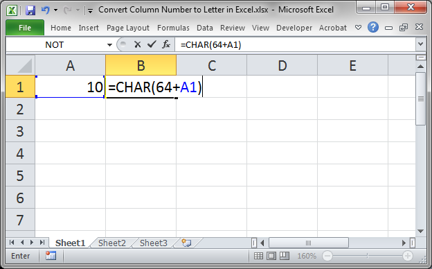
The formula:
=CHAR(64+A1)
A1 is the cell that contains the number of column for which you want to get the letter.
Result:
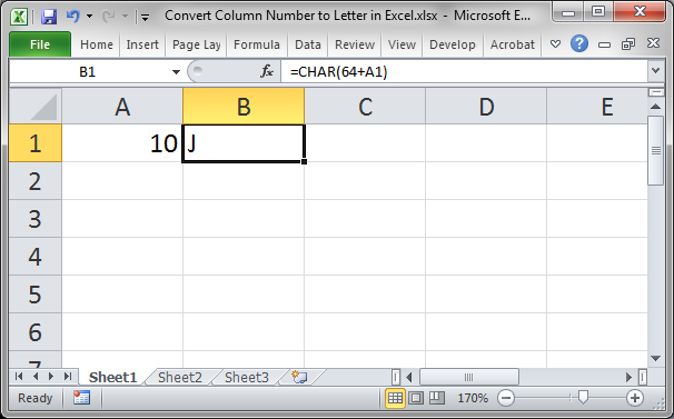
You could also write this formula like this:
=CHAR(64+10)
You just have to input the number for the column directly in the formula.
The CHAR() function gets a letter based on its number as defined by the character set of your computer; though, you don't need to know that to use this function.
Using COLUMN()
If you are creating a dynamic formula, you might want to automatically figure out the letter of a specific column for use in another function, such as the INDIRECT() function.
In this case, you can use the COLUMN() function to get the number of either a specific column or the current column:
=CHAR(64+COLUMN(A1))
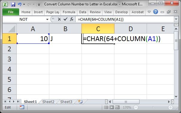
This would get the letter for the column for cell A1, which is A.
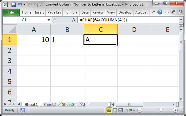
Remove the cell reference from the COLUMN() function and you will get the letter of the current column.
=CHAR(64+COLUMN())
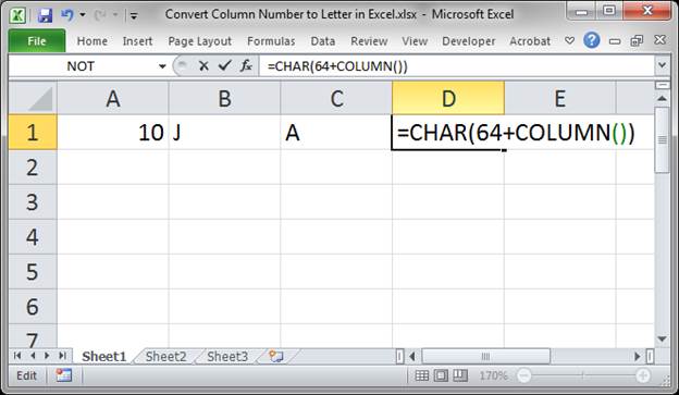
Result:
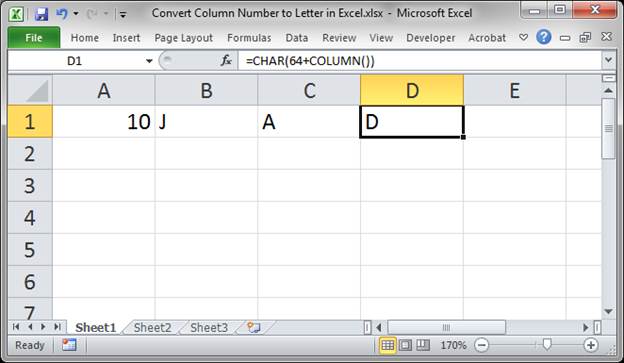
Remember though, this will only work for columns A to Z and, in some cases this might not work depending on the localized settings of the computer. The next example does not have these limitations.
More Complex Formula - Works For All Columns
This example is more versatile in that it works for all of the columns in Excel, but it is slightly more complex.
The formula:
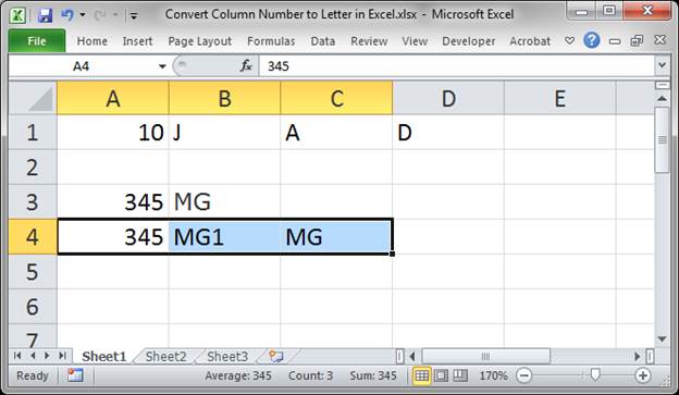
=SUBSTITUTE(ADDRESS(1,A3,4),"1","")
A3 is the example cell here that contains the number of the column for which we want to get a letter(s).
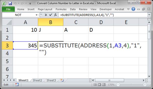
Result:
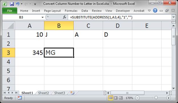
This formula uses the SUBSTITUTE() and ADDRESS() functions to get the column letters. This is a neat little trick that allows you to get the letters for any column using only a number as the reference for it.
The ADDRESS() function gives us the address of a cell based on a column and row number and the SUBSTITUTE() function replaces the number part of the cell reference with nothing, which removes the number. If you want to see this in Excel, just split these two functions into their own cell and look at the results:
Using COLUMN()
(this is almost the same as the COLUMN() section above, just with the new formula)
If you are creating a dynamic formula, you might want to automatically figure out the letter of a specific column for use in another function, such as the INDIRECT() function.
In this case, you can use the COLUMN() function to get the number of either a specific column or the current column:
=SUBSTITUTE(ADDRESS(1,COLUMN(A3),4),"1","")
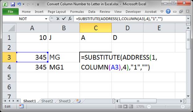
This will get the letter for the column for the cell reference A1, which is A.

You can also remove the cell reference from the COLUMN() function to get the letter(s) for the column in which the formula is currently placed.
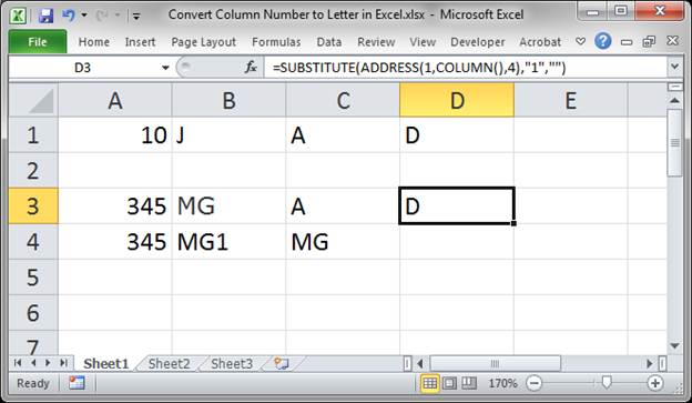
=SUBSTITUTE(ADDRESS(1,COLUMN(),4),"1","")
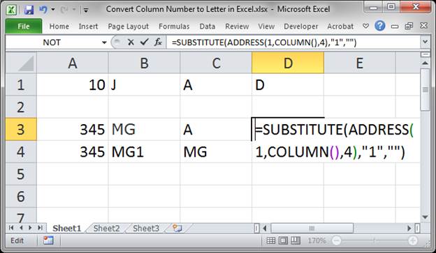
This will return D because the formula is in column D.
These last couple examples might seem trivial, but they are very helpful when you are copying the formula to a cell and column that is unknown, as in you don't know in which column the formula will be when it is used or copied.
Notes
This is a powerful thing to be able to do in Excel, get column letter(s) from their number. You won't use this every day and it might not help basic Excel users but, for all of you who want or need to take Excel to the next level, save this tutorial, especially for the second formula, the one that uses the SUBSTITUTE() and ADDRESS() functions.
Make sure to download the attached workbook so you can work with these examples in Excel.
Question? Ask it in our Excel Forum
Excel VBA Course - From Beginner to Expert
200+ Video Lessons 50+ Hours of Instruction 200+ Excel Guides
Become a master of VBA and Macros in Excel and learn how to automate all of your tasks in Excel with this online course. (No VBA experience required.)
Tutorial: How to convert a month's name, such as January, into a number using a formula in Excel; al...
Tutorial: Convert roman numerals to regular numbers (arabic) and also how to convert regular number...
Tutorial: 5 simple tips to evaluate any complex formula in Excel! These tips combine to give you th...
Tutorial: Make a particular worksheet visible using a macro in Excel. This is called activating a wo...
Tutorial: Find the Min or Max value in a range and, based on that, return a value from another rang...
Tutorial: Use a function in Excel to get the number of the day in a week, from 1 to 7. This allow...
Subscribe for Weekly Tutorials
BONUS: subscribe now to download our Top Tutorials Ebook!
Excel VBA Course - From Beginner to Expert
200+ Video Lessons
50+ Hours of Video
200+ Excel Guides
Become a master of VBA and Macros in Excel and learn how to automate all of your tasks in Excel with this online course. (No VBA experience required.)