Vlookup to Return All Matching Results

Here is an Excel formula that will act like a Vlookup that returns every matching result from a list.

Note: all formulas below are array formulas and so must be entered using Ctrl + Shift + Enter.

Sections:

The Formula

Formula That Hides Errors

Notes

The Formula

=INDEX($B$1:$B$7, SMALL(IF($A$1=$A$1:$A$7, ROW($A$1:$A$7)-ROW($A$1)+1), ROW(1:1)))

This is an Array Formula and so you must enter it into the cell using Ctrl + Shift + Enter.

This is a confusing formula so let me break it down for you.

First, there is no Vlookup function in there; the title of the tutorial says Vlookup because that is what most people understand, instead of "Index Array Formula to Return all Results."

What to Change to Work for Your Example

$A$1:$A$7 is the range reference that contains the values that you search through. You will need to change this in two locations within the formula.

$B$1:$B$7 is the range reference of the data that you want to return. This should be the same shape and size as the first range reference above.

ROW($A$1) contains the range reference of the very first cell in the data set through which you will search.

$A$1=$A$1:$A$7 the $A$1 part of this section contains the cell that you will use to lookup data. You can keep this as a cell reference or you can hard-code a text or number value in here. For text, wrap it with double quotation marks like this: "red" but for numbers you do not need to put quotation marks around it. In this example, it is the first cell in the lookup column, but it could be any cell within the worksheet or workbook, it doesn't matter where it is.

Here is an example of the code where this part is hardcoded for the text "red":

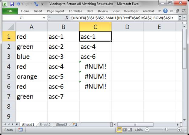
=INDEX($B$1:$B$7, SMALL(IF("red"=$A$1:$A$7, ROW($A$1:$A$7)-ROW($A$1)+1), ROW(1:1)))

ROW(1:1) should always be this for the first formula and it should be left as a relative cell reference (without dollar signs). This is important because this is what tells the formula which value in the list to return. When you copy the entire formula down, the number should increment by 1; ROW(1:1), ROW(2:2), ROW(3:3), etc. So, if you have three results for the text "red" this part of the formula says to return result 1, result 2, result 3, etc. Basically, leave this part alone and you should be OK.

Copy the formula down: you will enter this formula into the first cell and make sure that it works like it should. Then select that cell and copy it down as far as you need to return all of the results in the list.

Here is what is looks like in Excel:

Formula That Hides Errors

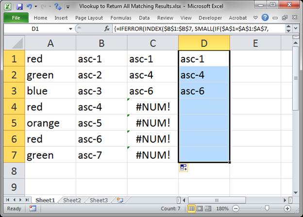
This formula has nice output instead of the ugly #NUM! error when a result isn't found.

This is the same base formula as above and so the details of that formula will not be covered again. The formula here is simply put within an error checking function.

Excel 2007+

=IFERROR(INDEX($B$1:$B$7, SMALL(IF($A$1=$A$1:$A$7, ROW($A$1:$A$7)-ROW($A$1)+1), ROW(1:1))),"")

In Excel 2007 and later we can use the IFERROR function to output a blank when there are no more results to return. This has the benefit of making it look like the list just appears as needed.

Excel 2003

=IF(ISERROR(INDEX($B$1:$B$7, SMALL(IF($A$1=$A$1:$A$7, ROW($A$1:$A$7)-ROW($A$1)+1), ROW(1:1)))),"",INDEX($B$1:$B$7, SMALL(IF($A$1=$A$1:$A$7, ROW($A$1:$A$7)-ROW($A$1)+1), ROW(1:1))))

This is for Excel versions prior to Excel 2007, such as Excel 2003.

This uses the same base formula as above except we have to use the IF function combined with the ISERROR function (there is no IFERROR() function in Excel 2003).

This looks confusing because it's quite long but it's really just the same base formula written twice. The ISERROR function checks if the formula creates an error or not and, if it does, it outputs a blank, but, if it works, then it moves to the second part of the IF statement, which contains the formula that we want to use.

It's a bit confusing, but this is how you have to hide errors for Excel 2003 and earlier.

Notes

This is a complex formula that involves a lot of moving parts; just remember that you don't have to understand every part of the formula in order to use it correctly, just edit the above formula, as specified, to fit your dataset.

Make sure to download the sample file to get these formulas in Excel.