Vlookup with a Range of Numbers in Excel

How to use the Vlookup function to return a result that falls within a range of numbers, such as a weight or quantity or even tests or grades.

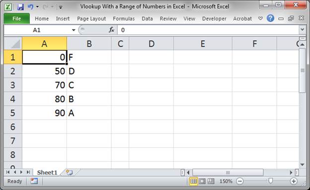
This allows you to, for example, return the letter A for a score of 90 - 100 on a test.

Here, it is assumed that you are at least partly familiar with the Vlookup function.  If you want to learn more about it, check out our Vlookup tutorial.

Steps to use the Vlookup Function with a Range of Numbers

1. Make sure that the data table that we want to search through is sorted in ascending order, which means that it is sorted lowest-to-highest.  Also, the value that we use to search through the table must be in the left-most column of the table.
   
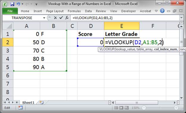
2. Enter the Vlookup function:
   
   
=VLOOKUP(D2,A1:B5,2)


   D2 is the cell that contains the lookup value or the value that we will use to search through the table to return a value.

   A1:B5 is the table where we will search for the value.

   2 is the number of the column in the lookup table from where we want to return a value.  1 would be the first column of the lookup table, which is also the column that contains the lookup values.

   We do not need to input anything in for the range_lookup argument, the fourth argument of the function.  However, if you want, you can enter TRUE for that argument, which is the default value.

   
3. Test it out.
   
   
   

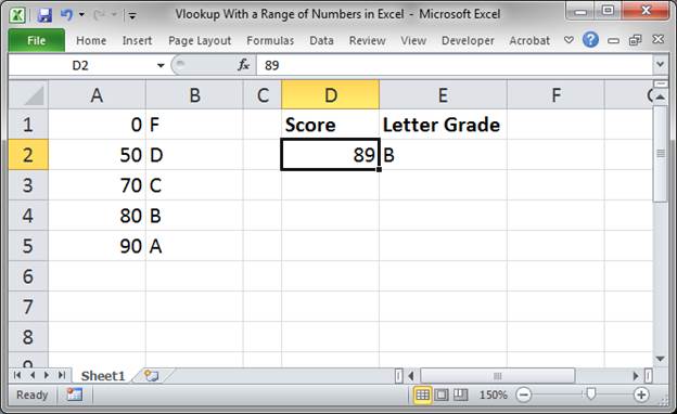
As you can see, as long as you are familiar with the Vlookup function, this is a very simple thing to do in Excel.  The most difficult part is to remember to sort the lookup table in ascending order.

Make sure to download the workbook that accompanies this tutorial so you can see this in action.