Round Numbers Up or Down in Excel
How to round a number up or down and also to a specified number of decimal places in Excel. This will allow you to create more useful mathematical functions and formulas.
Don't forget to download the accompanying workbook to follow along.
Sections:
Round a Number to a Specified Number of Digits in Excel
Round a Number Up in Excel
We will use the ROUNDUP() function to do this.
Round a Number Up to the Next Whole Number
=ROUNDUP(A2,0)
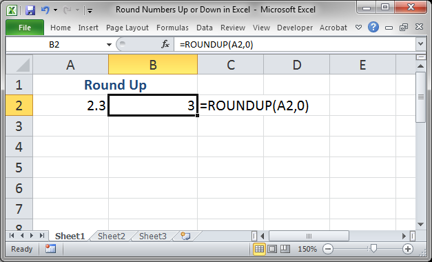
The first argument is the cell that contains the number that you want to round, A2, and the second argument is to how many decimal places you want to round the number. If you put 0 for the second argument that means that you want to round up to the nearest whole number (integer).
Round a Number Up to So Many Decimal Places
Here we will round up to a specified number of decimal places.
Let's say we have 2. 547 and we want to round to two decimal places, we do this:
=ROUNDUP(A3,2)
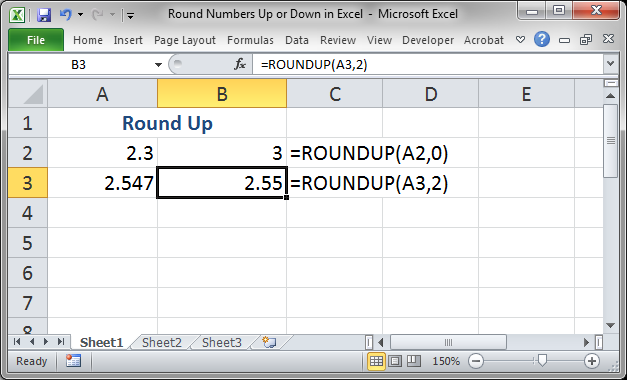
A3 is the cell with the number to round and 2 is put into the second argument to tell the function to round to the second decimal point.
Rounding Negative Numbers "Up"
This works like the previous examples except that we have negative numbers.

Technically, this is rounding the numbers down, but the function gives the exact same result as for the positive numbers, simply with a negative sign in front. Try not to get confused with this.
Round Up to the Nearest 10, 100, Etc.
You can also round a number up to the nearest value to the left of the decimal place if we use a negative number for the second argument in the ROUNDUP function.
Let's round 15 to the nearest ten and then 174 to the nearest hundred.
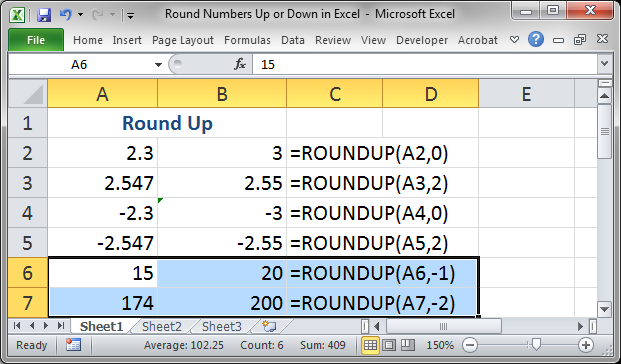
Note that we used -1 and then -2 for the second argument of the function.
If we use negative numbers, we get a similar result, though negative.

Round a Number Down in Excel
We use the ROUNDDOWN() function to do this. This works exactly like the ROUNDUP function except that it rounds the numbers down.
Round a Number Down to the Nearest Whole Number
=ROUNDDOWN(A9,0)
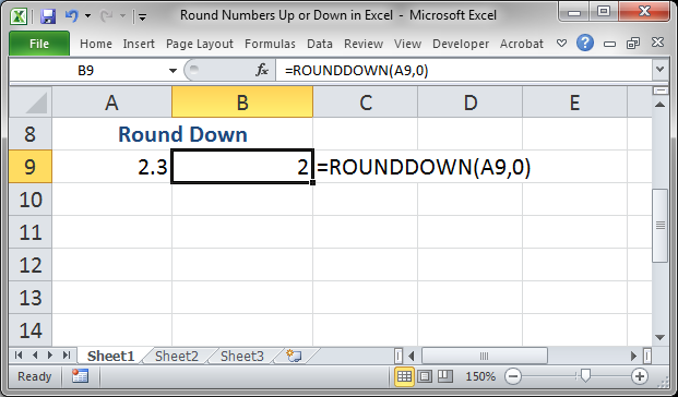
A9 is the cell that contains the number to round down and the 0 is to how many decimal places you want to round the number. If you round to 0 (zero) decimal places, that rounds the number down to the nearest whole number.
Round a Number Down to so Many Decimal Places
Round down to a specified number of decimal places. This time, we tell the function to how many decimal places it should round; to do this, change the 0 to whatever number you want.
=ROUNDDOWN(A10,2)
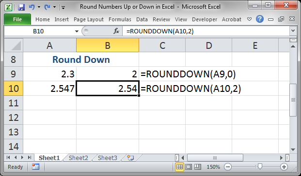
Here, we are rounding the number 2.547 down to two decimal places. As such, we place a 2 in the second argument for the ROUNDDOWN function.
Round Negative Numbers "Down"
This works exactly like the previous examples except that we are now using negative numbers instead of positive numbers.
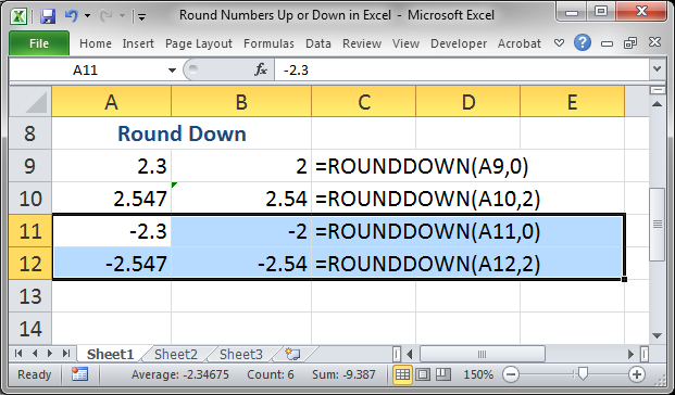
Technically, this rounds the numbers up, but, try to remember that it works exactly the same as when rounding positive numbers except that there is a negative sign in front of the numbers. This is the same as for the ROUNDUP function.
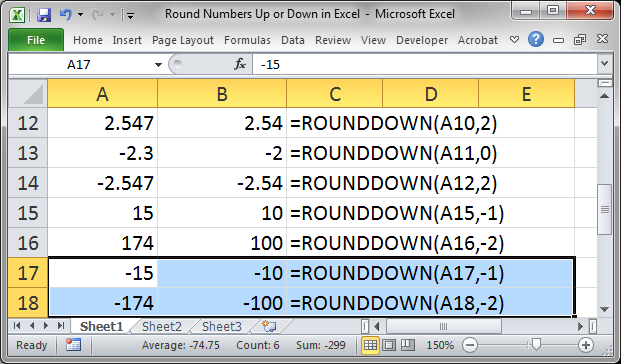
Round Down to the Nearest 10, 100, Etc.
You can also round a number down to the nearest value to the left of the decimal place if we use a negative number for the second argument in the ROUNDDOWN function.
Let's round 15 down to the nearest ten and then 174 down to the nearest hundred.
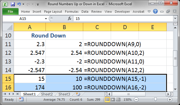
Note that we used -1 and then -2 for the second argument of the function.
If we use negative numbers, we get a similar result, though negative.
Round a Number to a Specified Number of Digits in Excel
Here, we use the regular ROUND function. This rounds numbers exactly like you would expect them to be rounded and just like you learned in school; that means that numbers are rounded to their nearest next value based on the number of decimal places to which you want to round.
Rounding Positive Numbers
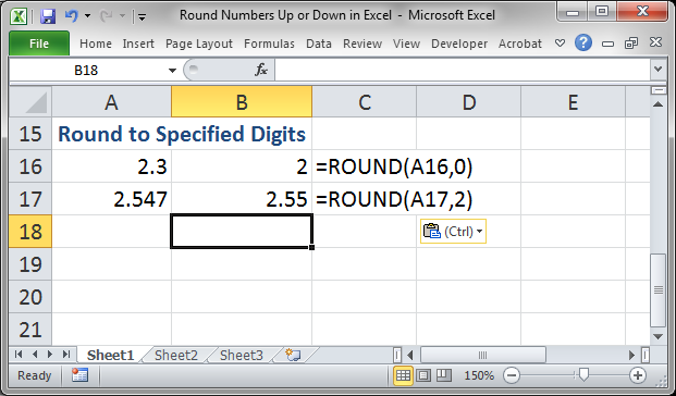
We use this function to round to the nearest whole number:
=ROUND(A16,0)
A16 is merely the cell that contains the number to be rounded. 0 is the second argument and that tells the function to how many decimal places we want to round the number. Remember that rounding to zero decimal places always means that we will be rounding to the nearest whole number.
To round to a specified decimal place, we use this:
=ROUND(A17,2)
This is the same formula as above except that we replaced the 0 with a 2. That means that the ROUND function will round to two decimal places.
Rounding Negative Numbers
You round these the same was as with positive numbers.
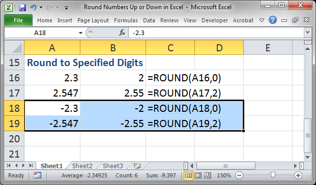
There is no different in how to use the function here, it is just that the numbers being rounded are negative.
Round to the Nearest 10, 100, Etc.
You can also round a number to the nearest value to the left of the decimal place if we use a negative number for the second argument in the ROUND function.
Let's round 15 to the nearest ten and then 174 to the nearest hundred.
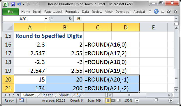
Note that we used -1 and then -2 for the second argument of the function.
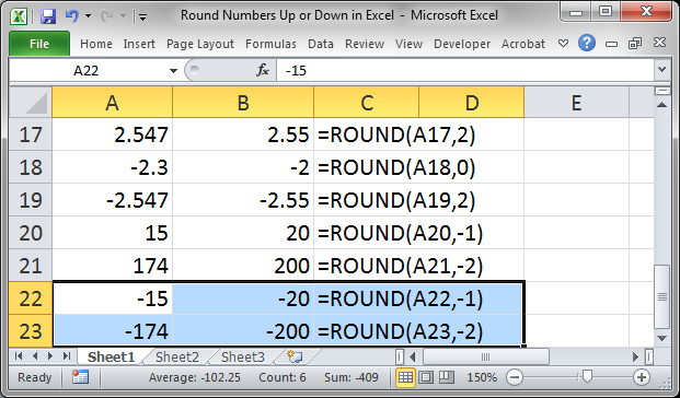
If we round negative numbers, we get a similar result, though negative.
Notes
The ROUND, ROUNDUP, and ROUNDDOWN functions are almost exactly the same. In fact, all three have the same arguments and these arguments are used in the exact same way. The difference is what each function does with the values you give them: regular rounding, rounding up, or rounding down.
Though these functions seem quite simple, because they are, you will need them when you are building complex calculations and formulas for Excel; as such, memorize these simple functions so you can add them to your list of tools in Excel.
Don't forget to download the accompanying worksheet to see these functions in action.
Question? Ask it in our Excel Forum
Excel VBA Course - From Beginner to Expert
200+ Video Lessons 50+ Hours of Instruction 200+ Excel Guides
Become a master of VBA and Macros in Excel and learn how to automate all of your tasks in Excel with this online course. (No VBA experience required.)
Tutorial: How to generate random whole numbers (integers) that are between two numbers. This allow...
Tutorial: How to convert a month's name, such as January, into a number using a formula in Excel; al...
Macro: This Excel macro automatically filters a set of data based on the words or text that are c...
Macro: Return the ISO Week Number in Excel with this UDF. This is a simple to use UDF (user defin...
Tutorial: This Excel tip shows you how to Sort Data Alphabetically and Numerically in Excel 2007. T...
Tutorial: In this tutorial I am going to show you how to update, change and manage the data used by ...
Subscribe for Weekly Tutorials
BONUS: subscribe now to download our Top Tutorials Ebook!
Excel VBA Course - From Beginner to Expert
200+ Video Lessons
50+ Hours of Video
200+ Excel Guides
Become a master of VBA and Macros in Excel and learn how to automate all of your tasks in Excel with this online course. (No VBA experience required.)