Make All Text Upper Case or Lower Case in Excel

How to quickly change all text to upper case or lower case in Excel.  This allows you to change the case of text without having to manually type in the text.

I will show you how to change the case of text and also how to make the results of the functions we will use actual text instead of function/formula output.

Also, check out our tutorial on how to capitalize first letter of every word in Excel.

Sections:

How to Quickly Make Text Upper Case in Excel

How to Quickly Make Text Lower Case in Excel

How to Make the New Text Actual Text instead of a Function

How to Quickly Make Text Upper Case in Excel

1. Go to the desired text.
   
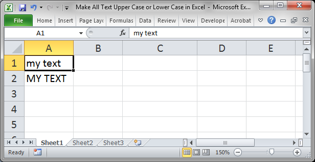
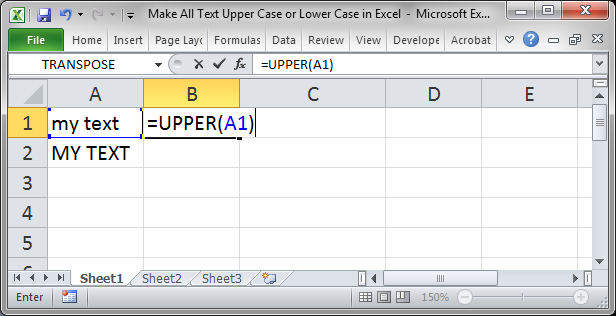
2. In another cell, type =UPPER(A1) where A1 is the reference of the cell that contains the text you want to make upper case.
   
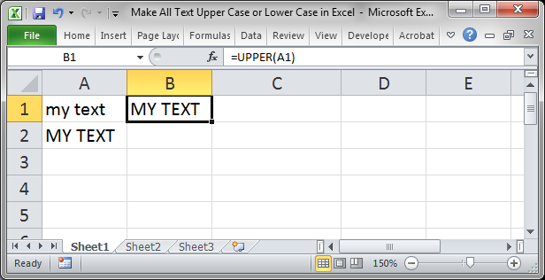
3. View the result:
   

How to Quickly Make Text Lower Case in Excel

1. Go to the desired text.
   
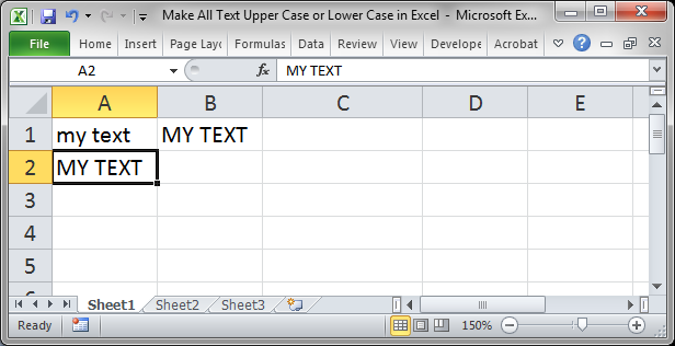
2. In another cell, type =LOWER(A2) where A2 is the reference of the cell that contains the text you want to make lower case.
   
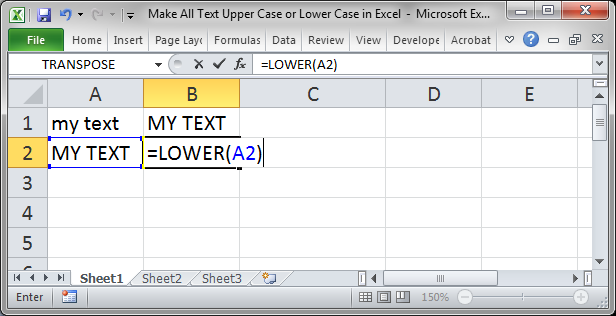
3. View the result:
   

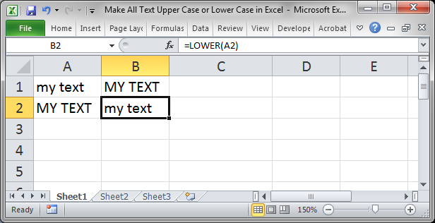
How to Make the New Text Actual Text instead of a Function

The problem with the above methods is that the output that we see that is now lower case or upper case is not actually text; it is the output of the UPPER and LOWER functions in Excel.  As such, we need to still have the original list of data in order to have the new list.

To remove the original list of data and keep the new list with either all upper case or lower case text we do this:

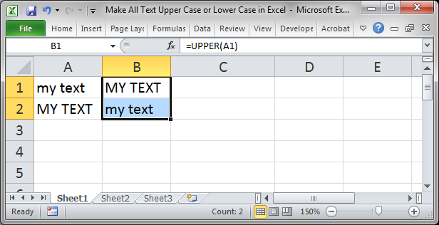
1. Select the output of the UPPER or LOWER function:
   
2. Hit Ctrl + C:
   
   
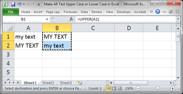
3. Hit Alt +  E + S + V and then Enter. (to remove the copy outline you can hit the escape (Esc) key after you hit Enter)
   
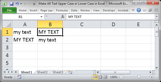
4. Now, we can delete the original column of data so that we only have one column of data.
   
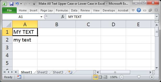
   Note that these cells, after step 3, contain only text.  There is no more UPPER or LOWER function contained within these cells.  This allows us to do whatever we want with the contents of the new list.

Notes

The UPPER and LOWER functions are great text manipulation functions that you can use to quickly clean or update lists of data.  These functions will save you a ton of time, especially with large lists of data.

Don't forget to download the accompanying workbook so you can follow the examples above.