Introduction to Using Filters to Refine Data in Excel

Filtering allows you to hide rows of data which you are not interested in so that you can easily look at the rows you want to see. Its as easy to use as sorting and can be basic or very complicated depending on how you use it.

In this tutorial I will just go through basic filtering. To filter a table you just select the column headings or the whole table itself then select Filter from 1 of 2 places. These are the same locations as the Sort feature was on the Home and Data tabs within the previous tutorial. The Filter function is always beside Sort by default in Excel. (Right-click then selecting Filter works slightly differently here and isnt as useful)

After selecting Filter, arrows should appear beside each of the columns in your selection. (Note: When filtering you always need column headings as the filter rules you apply do not affect the first row of your selection)

For this example I am going to filter out the surname Jackson. To do this I select the down arrow beside the Surname column heading. The following menu appears:

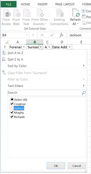
To filter all you do is untick the values you want to ignore. So as I wanted to ignore Jackson I unticked the box beside it. Notice how Jackson is only shown once here but appears twice in my table. This is because only distinct values are shown as filter options.

Alternatively I could have unchecked select all and then checked only the ones I want to see. It doesnt really matter which way round you do this, it all depends on the data set, what you are looking to filter and which is the quicker option. After you finish selecting your filter, click ok and the table will update. My table now appears like so:

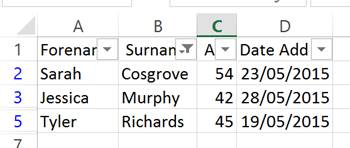
Rows 4 and 6 are now hidden. The filtered row numbers now turn blue to indicate filtering has been applied on those rows. There is also a filter symbol beside the column used to filter the data. As another example I will filter the Date Added column. Like before I just select the down arrow beside the Date Added column. I get the following menu:

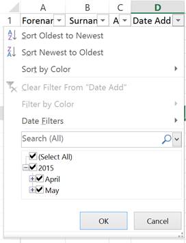
Whats cool about date formatted columns is that the filtering can be expanded to individual days or contracted to individual years. If I filter only rows with a date added in April I get the following:

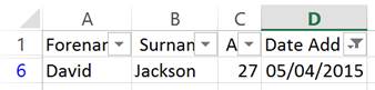
All the other rows have dates in May.

Number and date filtering also have more advanced features as they can be numerically evaluated. So for example if I select filtering on the Age column this time I can do a basic filter via the checkboxes like before but I can also select Number Filters to filter the table based on the numeric values of the Age column.

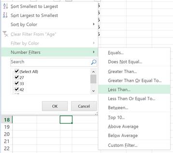
I could filter where Age is less than 30 for example but this is getting into the more advanced filtering options and involves setting filter rules which we will discuss in a later tutorial.