Ignore Blanks in a Data Validation List in Excel

I will show you 3 ways to remove the blanks from a Data Validation dropdown menu in Excel. All 3 methods are multi-step, but there is no way around this.

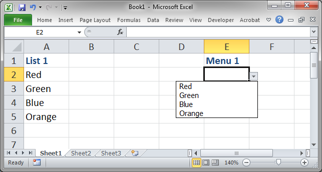
Here is the issue:

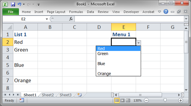
3 ways to Remove Blanks from a Data Validation Dropdown Menu List

Sorting Method (easy)

Remove Blanks Quickly (easy)

Complex Formula (Older Excel Versions) (complex)

Excel 365 Dynamic Array Formula to Remove Blanks (quite easy)

Conclusion

Sorting Method

The sorting method is quite simple and does not require a new list of data.

First, select the data from which we want to remove blanks:

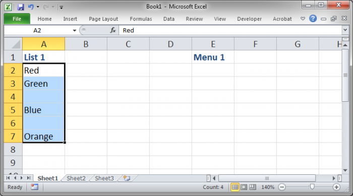
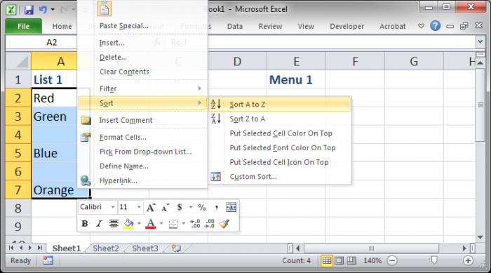
Right-click > Sort > Sort A to Z:

The sorted result:

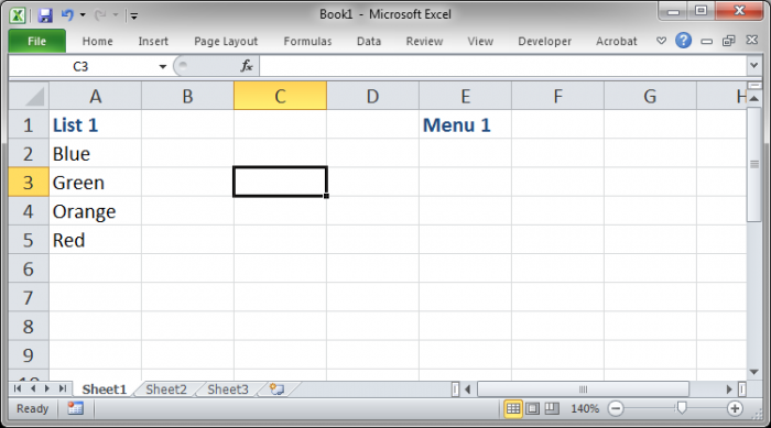
Now, all the blanks are at the bottom and it's easy to create a list without blanks:

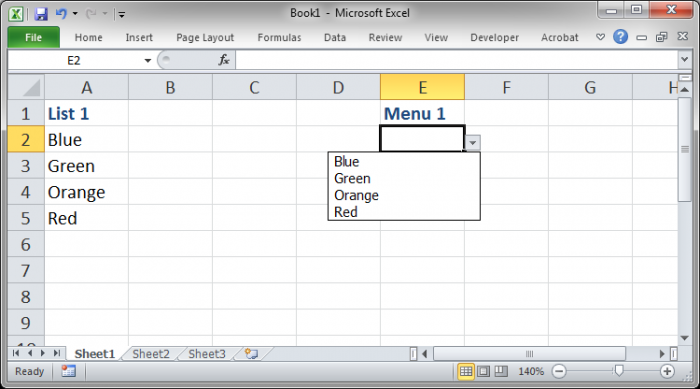
Note that I recreated the Data Validation list after the sorting, otherwise there would be two blanks at the bottom of the list.

Remove Blanks Quickly

This method will delete all of the blanks in a list and it is very easy to use.

First, we select where our list is:

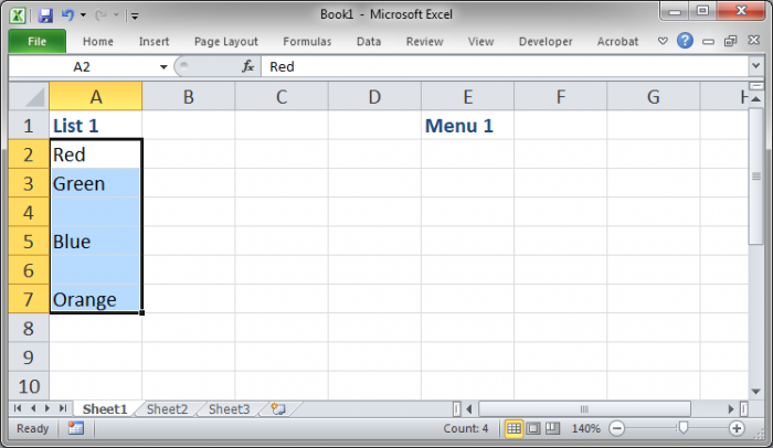
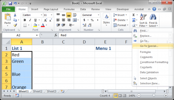
Then go to Go To Special.... In Excel 2007 and later go to the Home tab and look to the right and click the Find & Select button and then you can see this option.

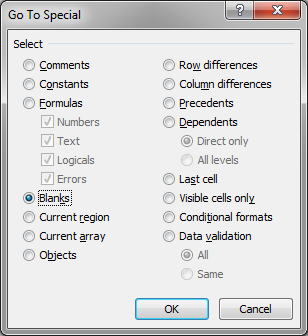
From the window that opens, select the Blanks option and hit OK.

You will see only the empty cells have been selected:

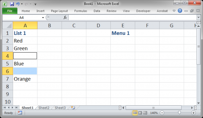
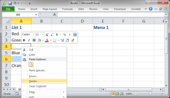
Now, right-click a selected cell, which will be a blank one, and click Delete.

Then, choose Shift cells up:

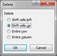
Hit OK and that's it!

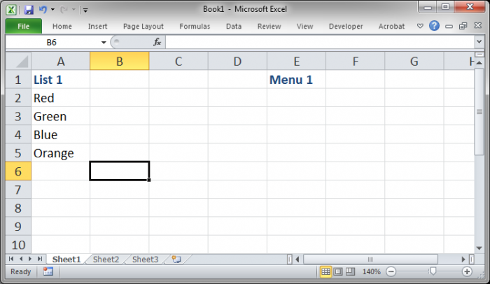
Now that all blanks are gone, we can create the Data Validation dropdown list without any blanks.

Complex Formula

This is the most complex and annoying way to create the list without blanks but it allows you to not have to touch the original list (although you could also achieve that by copy/pasting the original list for the previous two examples).

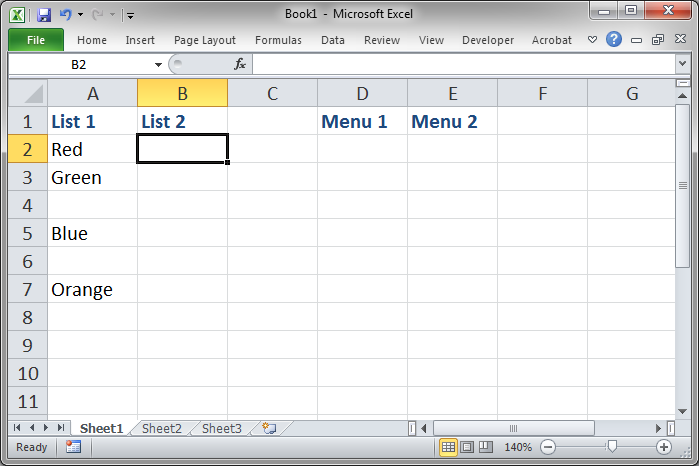
We start-off with this example:

Then we need to use the below formula to generate the new list:

=IFERROR(INDEX($A$2:$A$7,SMALL(IF(ISTEXT($A$2:$A$7),ROW($A$1:$A$6)), ROW(A1))),"")

We put this formula into cell B2 and use Ctrl + Shift + Enter to put it into the cell.

You MUST enter the formula into cell B2 in this way, instead of just hitting the Enter key, or it will not work.  That is because this is an Array Formula, which just means that it is very powerful/a pain in the butt.

Once you put this formula into cell B2 using Ctrl + Shift + Enter, copy the formula down the column and you will get this result:

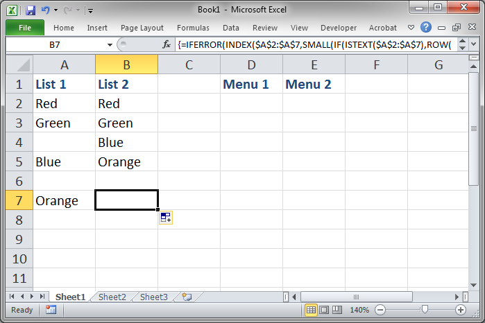
And BAM now we have a pretty list without any blanks!

Now, let me tell you what you need to change in the above formula so that it will work with your data set.  I'm not going to explain every element of the formula though, just what you need to change to make it work for you!

Here is our formula again:

=IFERROR(INDEX($A$2:$A$7,SMALL(IF(ISTEXT($A$2:$A$7),ROW($A$1:$A$6)), ROW(A1))),"")

You need to change where it says $A$2:$A$7 (it appears twice in the formula) to the column and row reference of your list.  If your list is in column D and goes from rows 2 to 35, you would change the above references to $D$2:$D$35

You also need to change where it says $A$1:$A$6  Notice that this is almost the same as the previous reference except that it starts in row 1 and only goes to 1 row below the end of the list.  So instead of going to row 7, the end of the list, it goes to row 6.  To update this for a new list in column D that goes from rows 2 to 35, we would change this range reference to $D$1:$D$34

This may seem confusing but there are only three range references that you need to change in this formula to make it work for you.

Note that this complex formula is made to work on data that is setup in a similar way, where it starts at the top of the worksheet and goes down the column.

Excel 365 Dynamic Array Formula to Remove Blanks

Remove blanks, sort, and return a unique list of values.

=SORT(UNIQUE(FILTER(A2:A7,A2:A7<>"")))

Conclusion

It is really annoying that Excel does not have a default feature to remove blanks from lists in Data Validation, remember the Ignore Blanks feature has nothing to do with this. 

But, using one of the three methods above, you will be able to get the nice list that you want.

Make sure to download the spreadsheet used in this tutorial so you can follow along and see the final result for yourself.