HLOOKUP in Excel

The Hlookup function allows you to scan a row from left to right in search of a value and then return the contents of a cell that is in the same column but below that row.

This is a "horizontal lookup" and works like the Vlookup or "vertical lookup" except that the Hlookup searches left to right instead of up and down.

Syntax

[] means the argument is optional.

Hlookup Sample

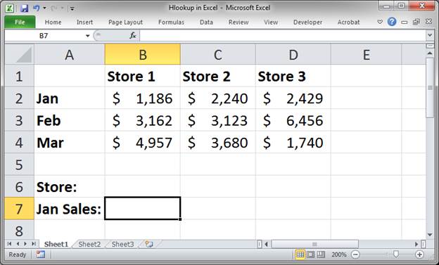
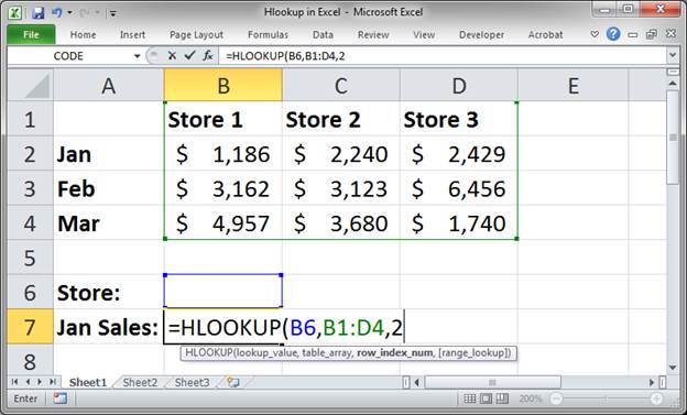
Here, we have a basic store sales setup and we want to get the January sales in cell B7.

(don't forget to download the accompanying workbook so you can follow along)

Steps to Use the Hlookup Function

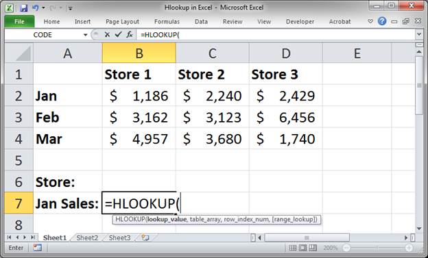
1. Type the function in the cell where you want the output to be displayed, and don't forget the opening parenthesis.
   
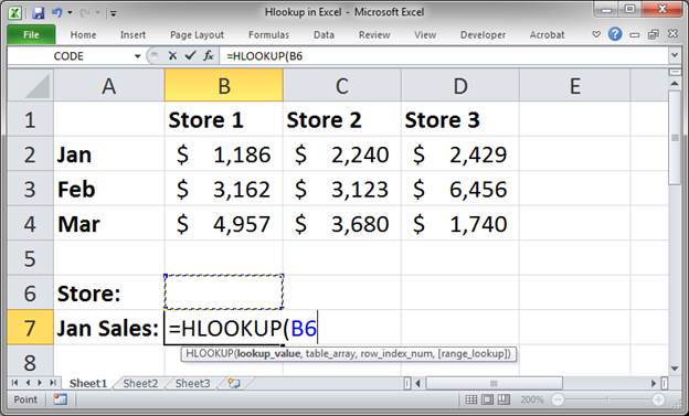
2. Fill-in the first argument, the lookup_value.  In almost all cases you will want to reference a cell where you will type in a value instead of hard-coding, or just typing, a value in for this argument.  If you do type a value in for this argument, make sure to put quotation marks around it like this "text" unless it is a number, which can be entered without quotes.  We will reference a cell, B6.
   
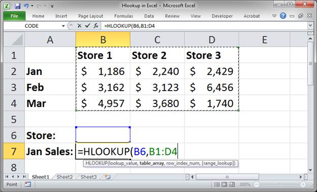
3. Type a comma to go to the next argument and then select the table in which you want to perform the search.  Make sure that the first row of the table is the row that you will use to search for the lookup_value.
   
4. Type a comma to go to the next argument.  Now, tell the function from which row you want to return data (remember that the first row is the lookup row).  Since January sales are the second row from the top row of the table_array, we input 2.
   
5. Now, we can leave this next argument empty if we want, but, in this case, we only want to make an exact match with the name of the store for the lookup_value and, to be honest, in most cases with lookup functions you will want an exact match.  As such, we put FALSE in for this argument (don't forget the comma before the argument).
   
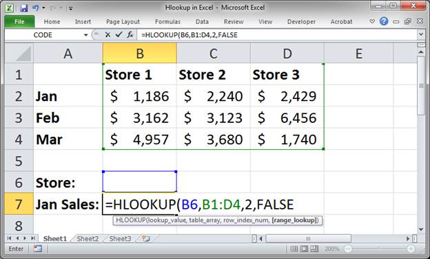
   Note that for this last argument, which can be TRUE or FALSE, we do not need to put quotation marks around it.
6. Hit enter and you are done.
   
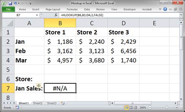
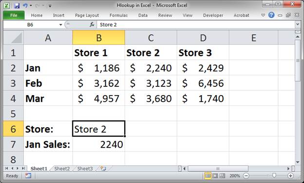
   We get an error because we haven't entered anything for the lookup_value yet.  You can follow this tutorial to remove the lookup error message.
7. Type a store name and we get our result!
   

Use the Hlookup Function with Numbers

If you want to search a list of numbers and return a specific number or the next highest value, you can do this with the Hlookup function.

Here is our sample data set for this example:

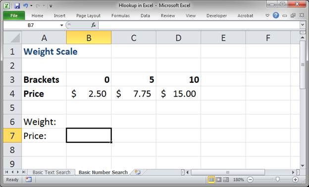
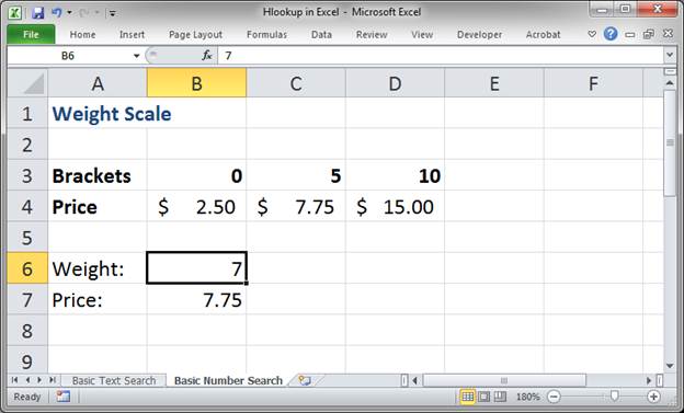
This sample will use the Hlookup to find the price of an item, let's say for shipping, based on its weight.  If the item is between 0 and 5 pounds, it costs $2.50 to ship; between 5 and 10 it costs $7.75 to ship; and 10 pounds and above it costs $15 to ship.

In order for this to work, the list must be sorted in ascending order with the lowest number on the left and the highest number on the right.

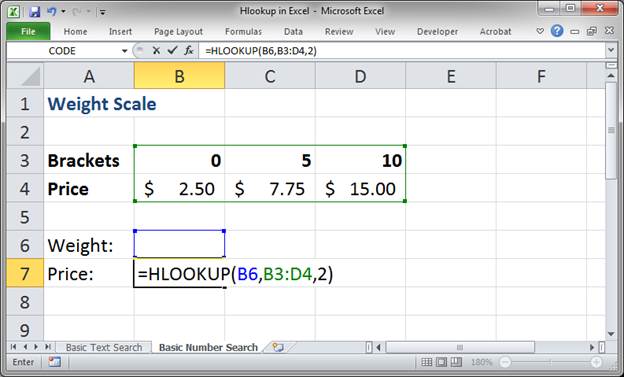
We input the Hlookup function just like above, except, this time, we either input TRUE for the last argument or leave it blank:

If we use nothing for the weight, we get 2.5:

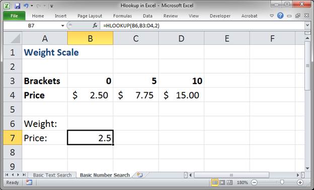
This happens here instead of an error because we did not put FALSE for the last argument of the Hlookup function and because the value in cell B3 is 0, which is considered the same as being empty in this case.

Now let's try some numbers in cell B6 and see what happens:

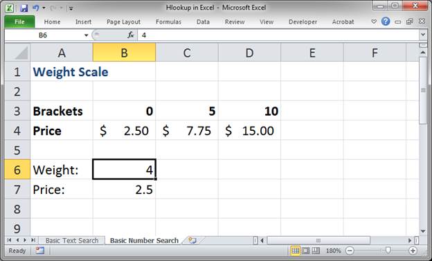
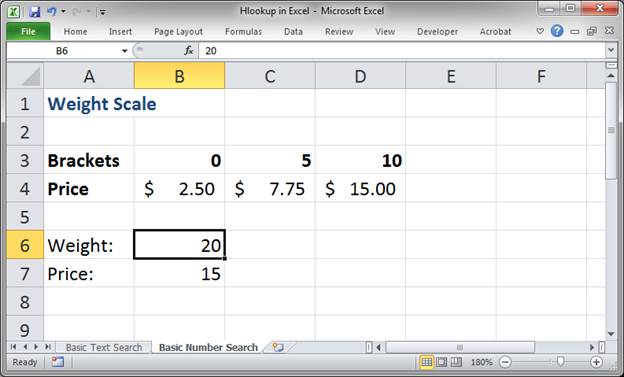
This should give you an example of how the Hlookup function will perform in this situation.

Notes

The Hlookup function works just like the Vlookup function except that the Hlookup goes left to right instead of up and down.

This function seems confusing at first but, trust me, once you use it a few times, it will be as easy as using the SUM function.

Make sure to download the accompanying workbook so you can follow this tutorial and see these Hlookup functions in action in the spreadsheet.