Highlight, Sort, and Group the Top and Bottom Performers in a List in Excel

How to highlight the rows of the top and bottom performers in a list of data.

This allows you to quickly identify who or what is performing well and performing badly.

In addition, you will learn how to sort this data so it appears next to each other so you can clearly see and compare the differences.

Sections:

Highlight Top and Bottom Performers

Sort Data so the Top and Bottom Performers are Adjacent to One Another

Notes

Highlight Top and Bottom Performers

1. Select the part of your data that you want highlighted.
   
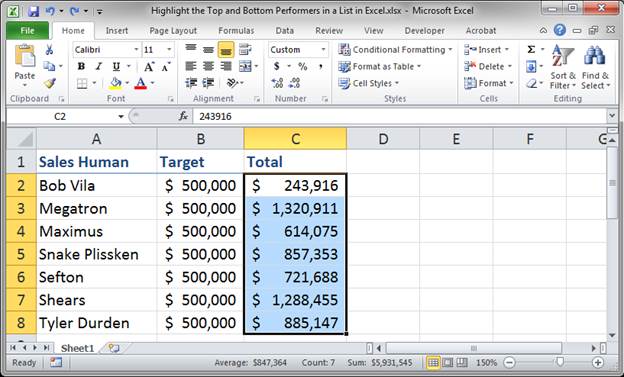
2. Go to the Home tab > Conditional Formatting > hover over Top/Bottom Rules and then you can select one of the default options from that list if it works for you or go to More Rules... for more options, which is what we'll do.
   
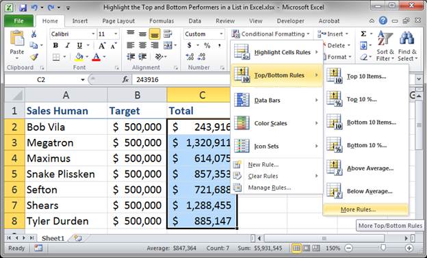
3. Once you click More Rules... you will see a small window like this:
   
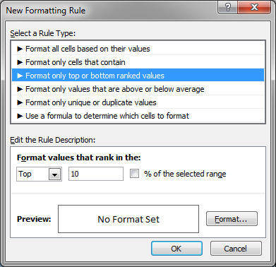
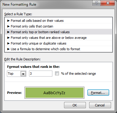
4. In the bottom of the window, you can choose to select the Top or Bottom from the menu and then how many you want highlighted or what percentage of the total you want highlighted.
   Once you've done that, click the Format... button to choose how the cells will look when highlighted.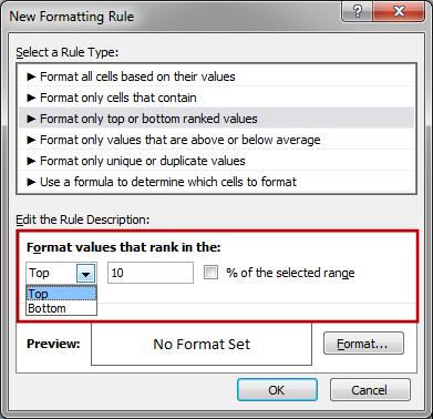
   
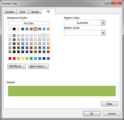
5. In the formatting window that appears, you can change A LOT to make the cells look however you want. Though, usually, all you need is to go to the Fill tab and select an appropriate color there. When you're done, hit OK.
   
6. You should see the first window again but with your formatting changes applied to the Preview section.
   
7. Hit OK and that's it!
   

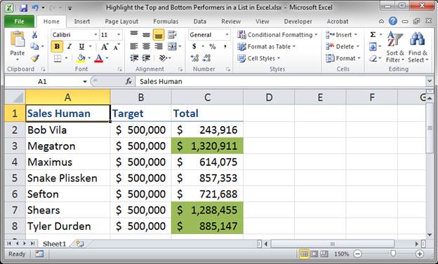
Now the Top 3 sellers are clearly listed.

Repeat for the bottom 3 and it will look like this:

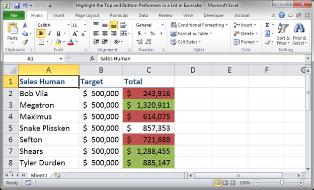
If this was a large list, all of these values might not appear on screen. In that case, sorting them so the top and bottom performers appear on top is important. Look to the next section to do that.

Sort Data so the Top and Bottom Performers are Adjacent to One Another            

To make the top and bottom values appear at the top of the list, we need to sort it in Excel.

1. Select the entire table of data and NOT just the single highlighted column.
   
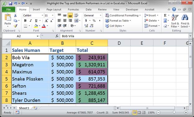
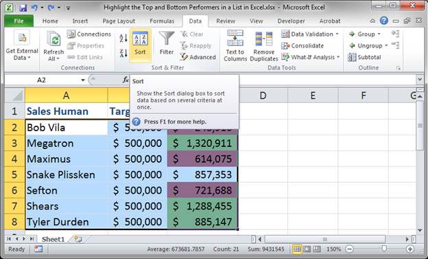
2. Go to the Data tab and click Sort.
   
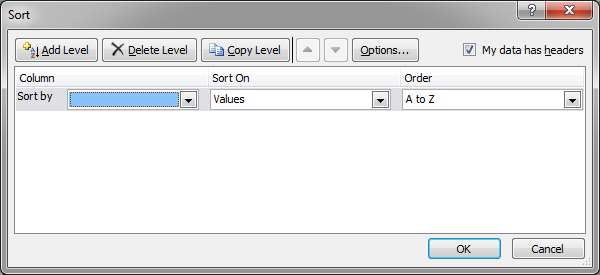
3. A window like this will open:
   
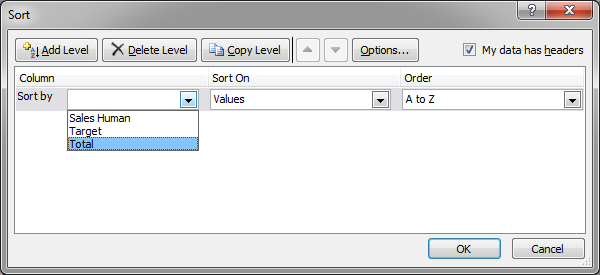
4. Click the first drop-down menu next to Sort by and select the column that has the highlighting, in this case the Total column. (Excel automatically names the columns by the headers they have.)
   
5. Go to the Sort On drop down menu and choose Cell Color
   
   
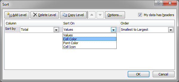
6. The Order menu area will have changed. Click the drop down menu for it that says No Cell Color and then choose the color that you want to be on top of the list.
   
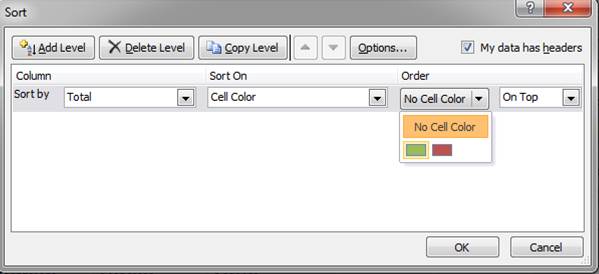
   Leave the second drop down menu in that section at On Top.
7. Your window will now look like this:
   
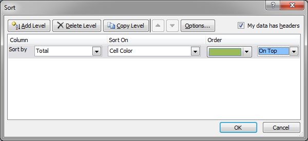
8. Now click the Add Level button and repeat Steps 4 to 7 for the next color that you want to show after the first color in the list. The window should now look like this:
   
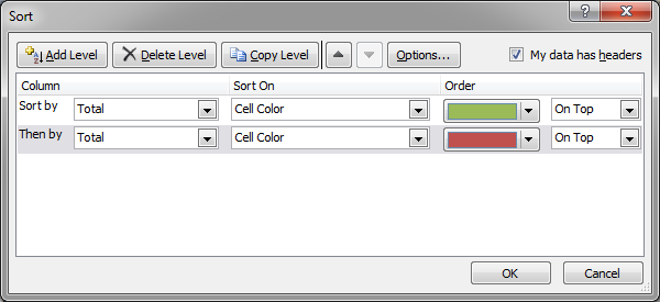
   Note that the colors will be sorted in the order in which they appear in this window. If you want to change that order, select a row from the Sort window and click the Up or Down arrow that is just to the left of the Options... button to change its position in sorting.
9. Repeat Step 8 as many times as is needed and then hit the OK button and you are done!
   Your data will now look like this:
   

Now you have a nice neat list with the top and bottom performers listed at the top of the list and everything else underneath that.

Sort Total Column Largest to Smallest

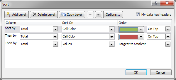
If you want to sort the Total column so the list will be in order of highest to lowest while still keeping the top and bottom performers at the top, you would add one more level to the Sort window that would look like this:

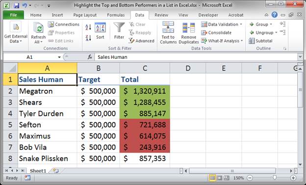
Then, our final result would be this:

Notes

To achieve this result, I used the Conditional Formatting features and Sorting by Color features of Excel. Though relatively simple to implement this setup, it makes analyzing data so much easier than just continually sorting up and down or scrolling to see the top/bottom performers.

This may seem like a lot of steps, but once you do it a few times, this will take you less than a minute to do to any size report or list of data.

Megatron is the best sales creature - it kinda makes sense since Megatron is a giant alien who can easily connect to computers, which means he would be great at sending out email campaigns and probably also Excel! (I just realized that he is not a Sales Human. ;) )

Make sure to download the sample file attached to this tutorial to work with this in Excel.