Group Data Together for Increased Readability in Excel
How to group data together or collapse it in order to focus only on the important data in Excel.
This allows you to take a big spreadsheet that contains a lot of data and make it more manageable and, therefore, easier to read and use.
This technique is different than simply hiding columns and rows, as that method does not make it easy to expand data back out where you can see it.
Sections:
How to Remove the Grouping Option from Your Data
Expand/Collapse All Groupings at Once
Group Data Together in Excel
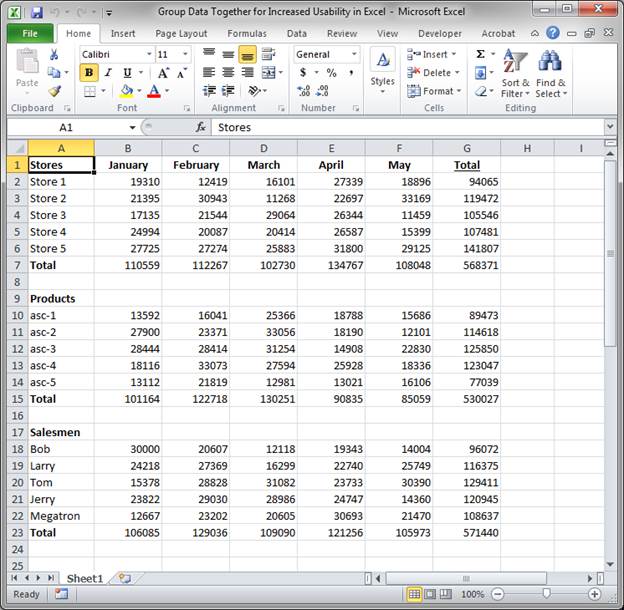
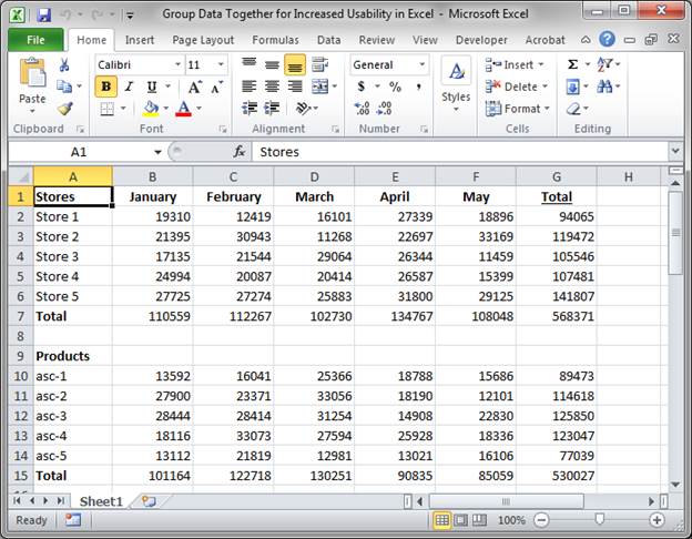
- Go to the worksheet that contains the data that you want to better view. The goal here is to collapse data so we can see what we want. We want to see only the heading and the total amounts.
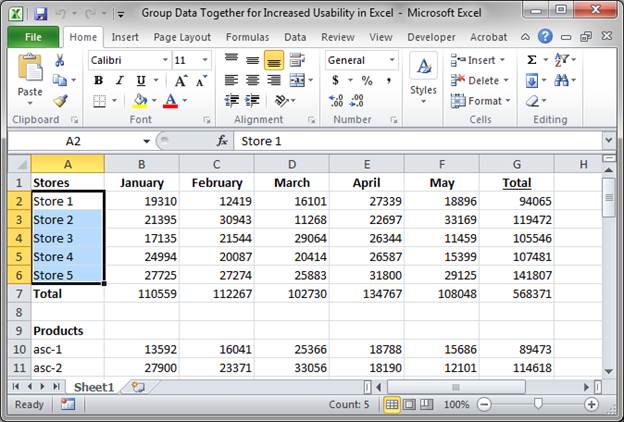
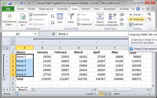
- Select the data in the rows or the columns that we want collapsed or hidden.
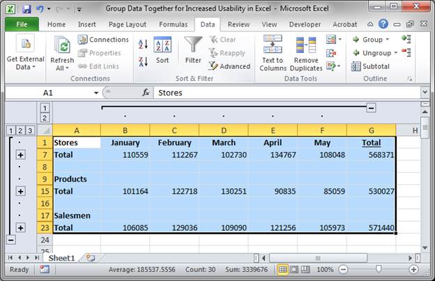
- Go to the Data tab and click the Group button all the way on the right (Shift + Alt + Right Arrow).
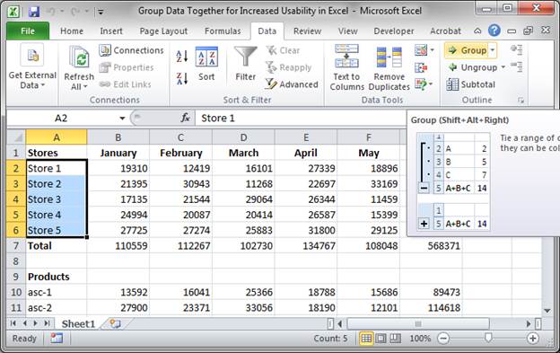
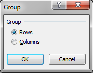
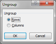
- In the window that opens, select Rows to group by rows. If we wanted to collapse columns, we would select Columns in this window.
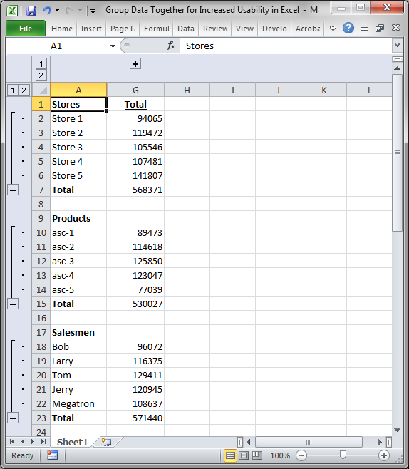
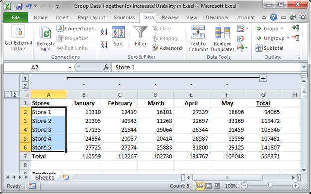
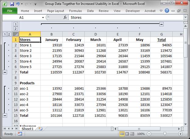
- Hit OK and you should see the worksheet now like this:
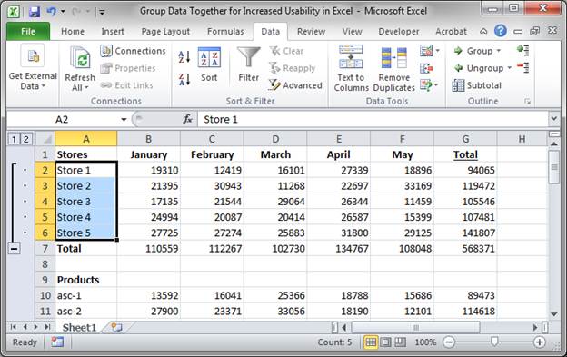
There is a line with a box under it next to the rows that we want to be able to easily collapse and hide.
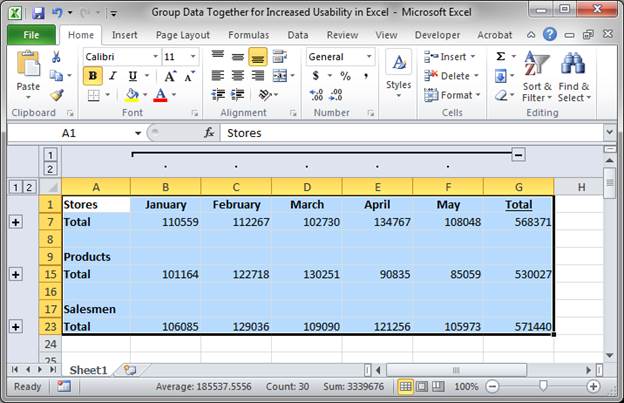
Click that box with the minus sign in it, the one that is just to the left of the header for row 7, and it will look like this: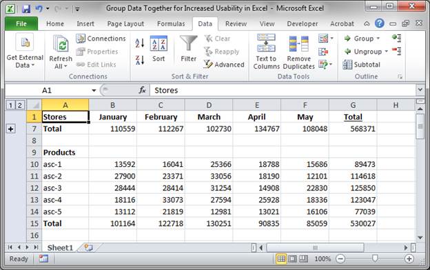
All of the data that we didn't need to see is now hidden and we can focus on the important stuff.
If you want to get the data back, just click the plus sign and it comes back: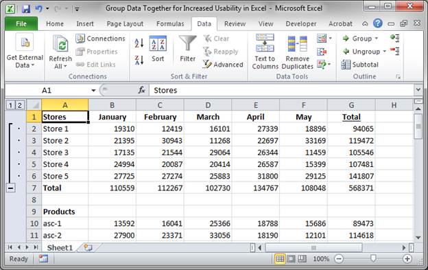
- Repeat Step 2-5 as many times as you need to collapse as much data as you need.
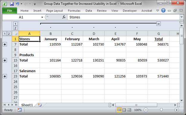
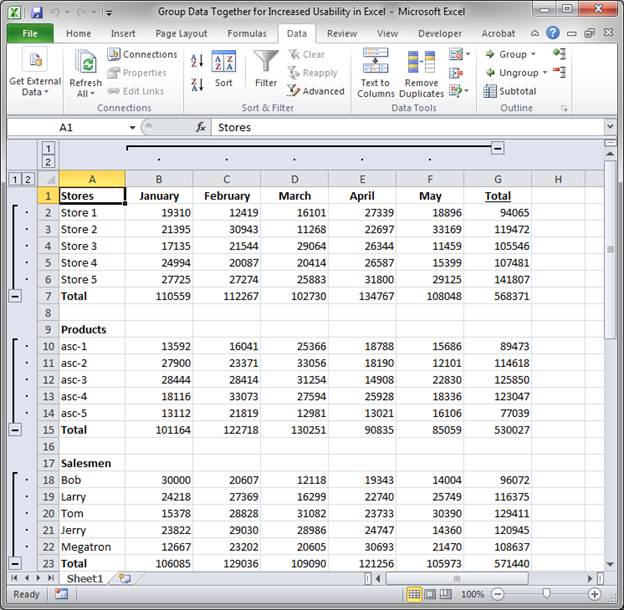
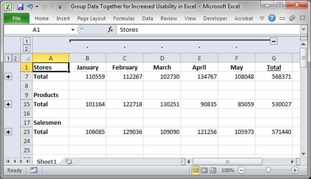
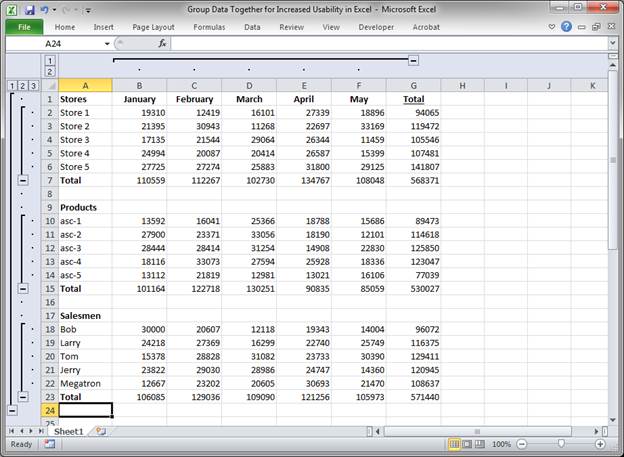
I repeated Steps 2-5 a few more times and now have grouped 3 sets of rows and one set of columns like this:
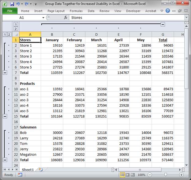
This allows me to see all of the data or just the totals by month like this:
Or just the totals by type like this:
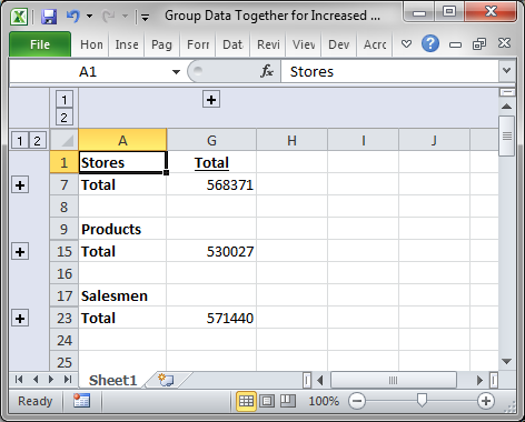
Or just the final total amounts for the three sections like this:
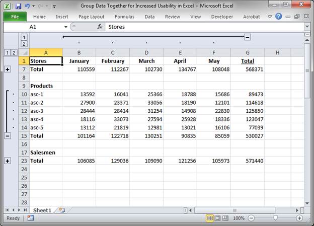
Also, sections can be controlled individually by clicking the Plus and Minus sign for that section:
As you can see, this allows you to generate many different views of your data quickly and efficiently without changing anything in your data.
Quickly Group A lot of Data
You can quickly group data on a worksheet, instead of doing it by hand, by using the Outline feature. This feature will guess how you want your data to be grouped together and do it all for you. Personally, I prefer the method described above since you have more control over your data but, sometimes, this method works well if you have a simple structured data set.
- Go to the worksheet that contains the data that you want to collapse/group.
- Go to the Data tab and look to the right and click the little arrow next to where it says Group and then click Auto Outline.
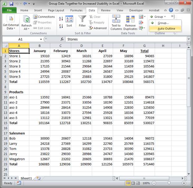
- If your data is setup in a way that Excel can easily understand, as is mine, then this should work just fine and you will get a result like this:
Here our data has been grouped by rows and also by columns.
If we collapse the data, it will look like this:

This way, we get the most important data and can drill down to see more data if we need to do that.
How to Remove the Grouping/Data Collapsing Option from Your Data
Remove Data Groupings from the Entre Sheet
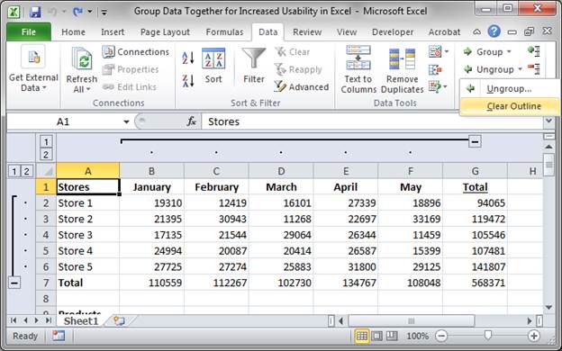
Select a cell anywhere on the worksheet and then go to the Data tab and click the arrow next to where it says Ungroup and then click the option Clear Outline. This will remove the groupings from the entire worksheet at once.
Remove Individual Data Groupings
Simply select the cells in the grouping that you no longer want to be grouped, you can select some or all of the cells in a specific grouping, and then go to the Data tab and click the Ungroup button (Shift + Alt + Left Arrow).
A window will open asking if you want to ungroup Rows or Columns. In this case, we want to ungroup rows, so just hit OK.
And that's it.
The cells that you selected will have their grouping removed but the other groupings on the worksheet will remain intact.
Expand/Collapse All Groupings at Once
Look to the boxes with 1 and 2 in them that are just to the left of column A and row 1.
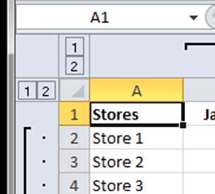
Click 1 to collapse all of the groupings for the rows or the columns; rows and columns are separately controlled.
Click the 2 to expand all of the groupings.
If you used layered groupings, explained below, you will see three numbers on the side instead of 2.
Add Layers of Groupings
Often you want to have layers of control so that you can see the individual data pieces if you want or you can just hide everything and see a summary.
You can add groupings to groupings the same way you added them in the first place.
Select the data that you want to be grouped.
Go to the Data tab and click the Group button and then, in this case, select Rows from the small window that appears and hit OK.
Now, we can collapse this data and focus on, say, a chart.
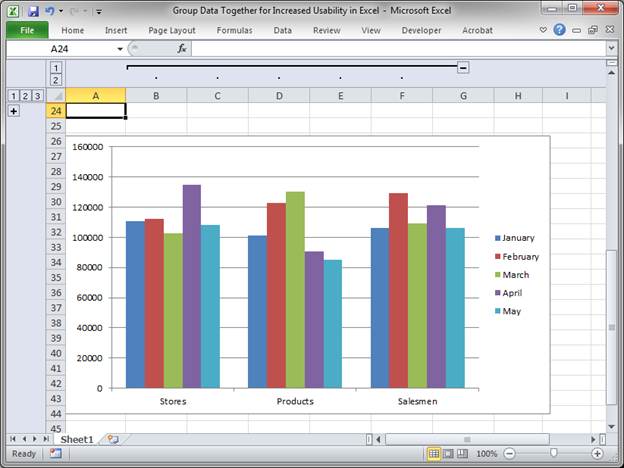
Or expand anything about which we need more information.
Notes
Adding groups to your data or collapsing it may seem odd, but it is a very helpful feature to use when analyzing a large amount of data on a spreadsheet. This allows you to organize your data so that you can focus on what is important but still be able to quickly and easily drill down into your data without messing up the existing spreadsheet.
If you have a chart in your worksheet and you hide or Group the data used to make it, the chart will be empty by default; here is a tutorial on how to Chart hidden data in Excel that will show you how to make it so that the chart will still work.
Download the spreadsheet that accompanies this tutorial so you can better see how grouping works and try it out in Excel.
Question? Ask it in our Excel Forum
Excel VBA Course - From Beginner to Expert
200+ Video Lessons 50+ Hours of Instruction 200+ Excel Guides
Become a master of VBA and Macros in Excel and learn how to automate all of your tasks in Excel with this online course. (No VBA experience required.)
Macro: Remove all data validation from a cell in Excel with this free Excel macro. This is a grea...
Tutorial: 3 ways to better use Slicers for Pivot Tables in Excel. These tips will show you how to a...
Macro: This free Excel macro allows you to display the print preview mode or window in Excel for ...
Tutorial: How to use parentheses in Excel in order to create more powerful formulas and functions. S...
Tutorial: How to sort a data set by multiple columns in Excel. This allows you to better organize ...
Tutorial: How to create dynamic charts that update automatically when new data is added to Excel. T...
Subscribe for Weekly Tutorials
BONUS: subscribe now to download our Top Tutorials Ebook!
Excel VBA Course - From Beginner to Expert
200+ Video Lessons
50+ Hours of Video
200+ Excel Guides
Become a master of VBA and Macros in Excel and learn how to automate all of your tasks in Excel with this online course. (No VBA experience required.)