Easily Input Complex Functions in Excel
In this tutorial I am going to show you how to easily input complex Functions in Excel.
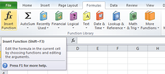
To insert a Function, select a cell then navigate to the Formula tab and click the Insert Function button.
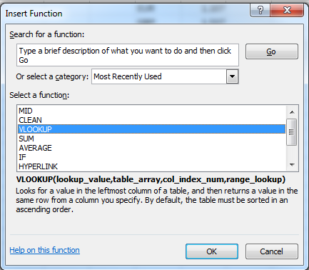
You then select the Function you wish to Insert and click ok (For this example I am going to insert the VLOOKUP Function).
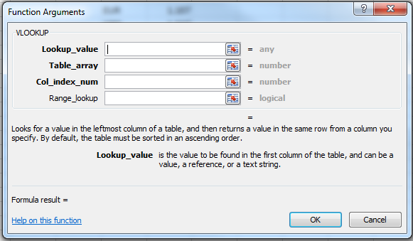
The following window opens:
Note: You can also use the Function Library section of the Formulas tab to get to this window too.
This is the window that lets you edit the Function Arguments before inserting it into the workbook. It is a really useful feature as it gives details about what the Function does, what data should be given for each argument and the data types of the arguments.
The first thing to look at when inserting a Function is the description to better understand how it works. Below the Argument boxes the VLOOKUP Function has the following description:

Below this is further detail about the current Argument you are editing. So as my cursor is in the Lookup_value Argument box, details on the Lookup_value Argument are given:

As you work down the Arguments boxes, a description for each will be shown at the bottom of the window. Now lets look at the Argument boxes themselves:

To the right of each box there is a hint for what type of data should go in each. Looking at the Vlookup Function above, the Lookup_Value Argument has the data type any. This means that any type of data can be entered here. This includes values, text strings and cell references. For this example I have selected the cell A2:

As my cell reference is a valid argument, the value of the argument is shown to right. (JPY)
Note: By clicking the button to the right of the Argument box you can shrink the pop-up window in order to better see the worksheet and select cells.


The next Argument (Table_array) has the data type number. This can be a bit misleading as a cell range is required here not a number. The clue here is the array part of the Argument name. This indicates that an array/or table of cells must be given as the Argument instead of a single value. If this isnt clear, always remember to read the Argument description:

The description specifically mentions a table of text, numbers, or logical values. This means a cell range should be given here like so:

Moving onto the next Argument (Col_index_num). Again this Argument has the data type of a number but it has num on the end instead of array. This means that only numbers can entered for this argument. If I entered Text here, I would get the #VALUE! error. This indicates that the value I have entered does not match the data type required for this argument:

Changing this to 2 fixes the issue as a number is required:

The last Argument (Range_lookup) for the VLOOKUP Function has the Logic data type. This means it only accepts either True or False as the Argument. It is important to read the description here to see how a True or False value will affect the Function:

Text Example
Another data type which isnt covered by the VLOOKUP Function is the text data type. If I insert a Function which manipulates text, such as the LEFT function:
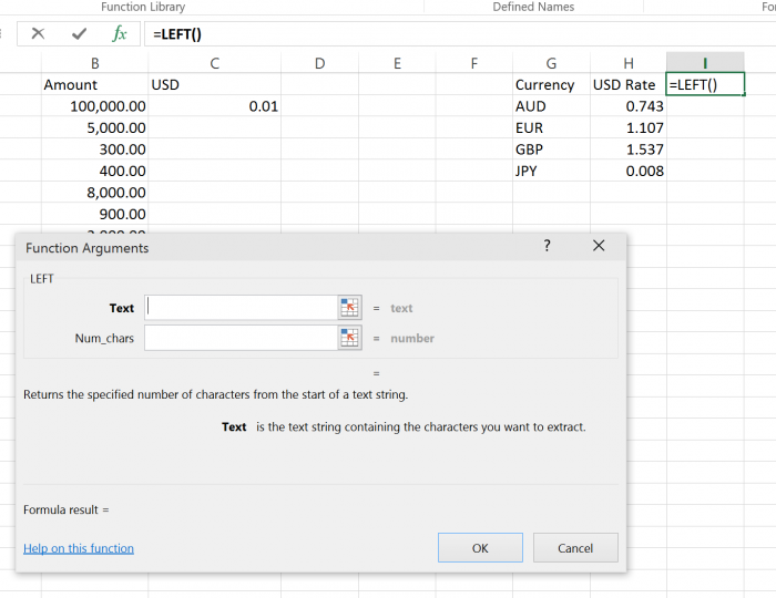
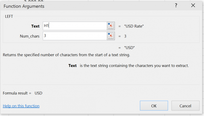
The data type for the first Argument is text and the description specifically mentions a text string. Note that text can also be represented by a cell reference, as long as the cell contains text:
Required Arguments
One final thing to note is that when the name of an argument is in bold, like Text above (or the first 3 arguments of the VLOOKUP) it is a required Argument. If it is not in bold then it is an optional Argument like Num_chars above.
Dont forget to download the accompanying workbook so you can follow along!
Question? Ask it in our Excel Forum
Tutorial: How to create a custom worksheet function in Excel. These are called User Defined Function...
Tutorial: Here, I'll show you a quick, simple, and effective way to fix formulas and functions in E...
Tutorial: Full explanation of the Vlookup function in Excel, what it is, how to use it, and when yo...
Tutorial: In this tutorial I will cover the basic concepts of Formulas and Functions in Excel. A for...
Tutorial: The OFFSET function in Excel returns a cell or range reference that is a specified number...
Tutorial: 5 simple tips to evaluate any complex formula in Excel! These tips combine to give you th...


