Formula to Delete the First or Last Word from a Cell in Excel

Excel formula to delete the first or last word from a cell.

You can copy and paste the formulas below for a quick fix and also learn how they work, if you're interested.

Sections:

Remove the First Word from a Cell

Remove the Last Word from a Cell

More Versatile Formulas - Prevents Errors

Notes

Remove the First Word from a Cell

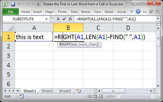
=RIGHT(A1,LEN(A1)-FIND(" ",A1))

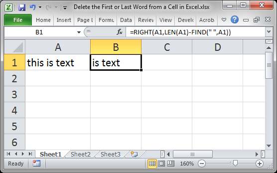
Result:

This assumes the text is in cell A1, change as needed for your spreadsheet.

Non-Space Characters

If your words use dashes or some other separator, just replace " " with whatever separator is used. If a dash is used, change that to "-" in your formula.

Explanation

There are three functions at work here: the RIGHT(), LEN(), and FIND() functions.

The RIGHT function is what gets the text from the right of the cell. This is needed because we are extracting all of the text except the first word; that means we need to get everything that is to the right of the first word in the cell.

The LEN and FIND functions are used to tell the RIGHT function how many characters on the right of the cell we want to get. The RIGHT function only extracts so many characters from the right of the cell.

To get everything except the first word, we need to find the space that separates the first word and the rest of the text. Use the FIND function, searching for a space " " to get the number of characters from the left of the cell until the first space. In the example above this returns 5. That is the number of characters that we want to remove from the cell.

To get the number that we want to keep, we need to use the LEN function to count all of the characters in the cell. The result of the LEN function is 12 because there are 12 characters in the cell.

In the formula above, we subtract the result of FIND from that of LEN, which is 12-5, or 7.

This tells the RIGHT function to get 7 characters from the right of the cell, which effectively removes the first word from the cell.

Remove the Last Word from a Cell

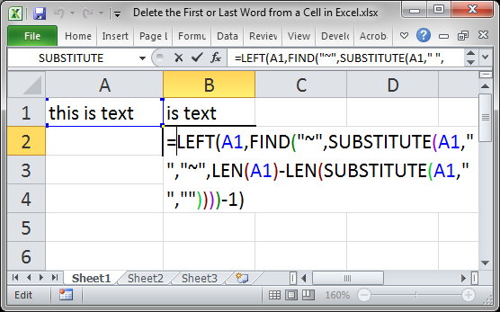
=LEFT(A1,FIND("~",SUBSTITUTE(A1," ","~",LEN(A1)-LEN(SUBSTITUTE(A1," ",""))))-1)

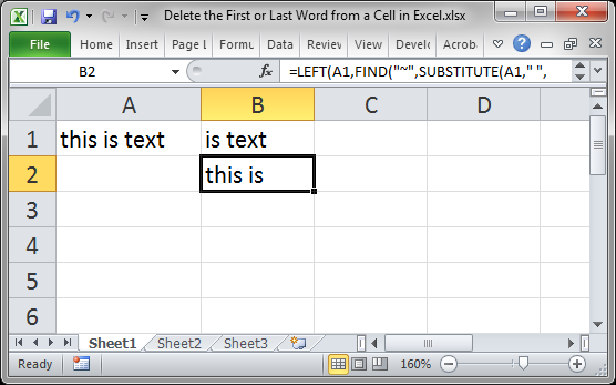
Result:

This assumes the text is in cell A1, change as needed for your spreadsheet.

Note: if your cells might have the ~ character in them, change that part of the formula to a character that won't be present in the cells.

Non-Space Characters

If your words use dashes or some other separator, just replace " " with whatever separator is used. If a dash is used, change that to "-" in your formula.

Explanation

This formula uses four functions: LEFT(), LEN(), FIND(), SUBSTITUTE().

This can be a bit confusing but you don't need to read this section in order to use the formula.

In order to remove the last word from the cell, we need to extract all of the other words to a new cell and this new cell will then not contain the last word. Basically, we are getting all of the words that are to the left of the last word, so we use the LEFT function.

To do this, we need to tell the LEFT function how many characters from the left of the cell that we want in the new cell, and that number can vary. The tricky part of the formula is what gets us this number.

FIND("~",SUBSTITUTE(A1," ","~",LEN(A1)-LEN(SUBSTITUTE(A1," ",""))))

This piece of the formula SUBSTITUTE(A1," ","") removes all spaces in the cell and then counts how many characters are left using the LEN function LEN(SUBSTITUTE(A1," ","")). From the example above, the result of this is 10.

It then counts how many characters are in the cell when the spaces are left in it: LEN(A1). The result is 12.

Then the formula subtracts the two above numbers to get 2 in this example. This number is the total number of spaces that are in the cell and this tells the other SUBSTITUTE function which space to replace; we want to replace the last space so we can find it more easily.

Using the number we just got, the SUBSTITUTE function is used again to replace the last space in the cell with ~ and then the FIND function is used to find that ~ and then the formula knows how many characters from the left of the cell the last space is.

The formula then subtracts 1 from that number since we don't want to include the last space in the new cell.

Now, we have the total number of characters from the left of the cell up to the space that comes before the last word in the cell and we can use the LEFT function to return everything except the last word.

If you are still a little confused, check out our tutorial on the SUBSTITUTE function in Excel

More Versatile Formulas - Prevents Errors

If you use one of the above formulas on a list and any of the cells in that list contains a single word, an error will appear.

To avoid any errors, we can use a simple IFERROR() function.

Formula 1:

=IFERROR(RIGHT(A1,LEN(A1)-FIND(" ",A1)),A1)

Formula 2:

=IFERROR(LEFT(A1,FIND("~",SUBSTITUTE(A1," ","~",LEN(A1)-LEN(SUBSTITUTE(A1," ",""))))-1),A1)

This says that if there is an error, output the contents of the original cell. Errors like this usually happen if there is only one word in the cell, so this would output that single word.

Read our tutorial to learn more about the IFERROR function in Excel and suppressing errors in general.

Notes

These formulas can be confusing. I recommend simply copy/pasting them into your spreadsheet and changing the cell references as needed.

To make the new range of values text instead of formulas follow this tutorial for converting formulas to values.

Make sure to download the sample file attached to this tutorial to get these examples in Excel.