Complex Structured References (Table Formulas) in Excel

If you don't already understand how structured references work or what they do, please read our tutorial on that: using formulas with tables in Excel.

Note: the examples below will show you how to make the references but won't necessarily show you useful real world examples. This is in an effort to teach the main concepts, which are, themselves, quite tricky.  If you want useful examples, simply wrap the ones in this tutorial in a SUM or AVERAGE function to see results.

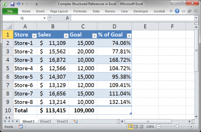
All examples are based on this table, which is named SalesData:

(Download the attached file to follow along with these examples.)

Sections:

Referencing Multiple Columns at Once

Referencing a Section of a Column

Reference a Section of the Table Across Multiple Columns

Notes

Referencing Multiple Columns at Once

Reference Multiple Separate Columns

You simply reference each column separately and put a comma between the references.

Reference Multiple Contiguous Columns

Two things here:

We reference two columns but separate them only with a colon :

Since we reference two columns next to each other, we must put another pair of brackets around them, which is why you see an extra one before Goal and an extra one at the end after % of Goal.

Reference the Intersection of Columns

This is the most complex method. Intersection is where two range references overlap.  In this example we would end up referencing the Goal column because that is the only column that is listed in both table column references.

There are two column range references here: SalesData[[Sales]:[Goal]] and SalesData[[Goal]:[% of Goal]] and they are separated using a single space and nothing more; that single space is important and this won't work without it.

The syntax of the column range references is the same as the Contiguous Column example above it.

Referencing a Section of a Column

You can reference particular sections of a column using the item specifiers:

#All, #Data, #Headers, and #Totals (explained in the tutorial that is linked to at the top of this tutorial)

Example:

This references the Totals row in the Sales column of the SalesData table.

Note that there is a comma between the item specifier and the column name.

Note also that there is an extra set of brackets surrounding the reference for the table; an extra bracket before #Totals and an extra one after Sales.

Using this method you can reference any part of the column by changing Totals to any of the item specifiers, such as Headers or All.

Reference a Section of the Table Across Multiple Columns

This combines what was learned in the Referencing Multiple Columns at Once section and the Referencing a Section of a Column section.

Reference the totals of the Sales column and the Goal Column:

There is the #Totals reference at the start and then a comma and then, instead of a single column reference, there is a multi-column reference.

If the two columns Sales and Goal were not touching, we would have to adjust the formula to look like this:

Though this looks complex, it merely follows the syntax rules laid out in the example above for Reference Multiple Separate Columns combined with referencing the section of a column.

Notes

These formulas, structured reference formulas for tables, can be quite tricky and confusing. This tutorial assumes that you have a basic understanding of how they work and, if you don't, then you should visit the tutorial that is linked to at the top of this tutorial so you know what is going on.

You should play around with these formulas and practice them until you get the hang of the syntax.  Nothing is really difficult, it's just that the syntax is different from the regular Excel syntax and that takes time to get used to.

Make sure to download the sample file for this tutorial so you can try everything out in Excel.  To make the formulas actually work and return a value, wrap them in a SUM or AVERAGE function.