Best Lookup Formula in Excel - Index and Match
A lookup using INDEX and MATCH is like a VLOOKUP without the restrictions. Index and Match lookups offer you freedom, to search to the left as well as the right and to perform more complex two way lookups with ease.
Performing an Index/Match lookup is confusing at first. Here, I'll show you how to do everything step by step.
(before you start, make sure to download the sample file for this tutorial so you can follow along with the examples below)
Sections:
Create a Lookup Using INDEX and MATCH
Create a Right-to-Left Lookup Using INDEX and MATCH
Create a Two-Way Lookup Using INDEX and MATCH
Create a Lookup Using INDEX and MATCH
This is how to create a basic lookup. This will be the simplest version of a lookup and it will work exactly like a Vlookup; it's important to start simple so you can get a feel for how we input the formula.
In the example below, we want to search a "Rank" column and have it return a value from the "Site" column.
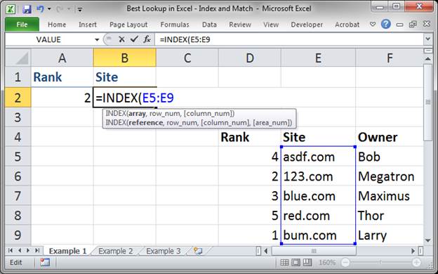
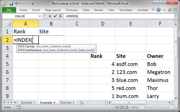
- First, type =INDEX(

- Select the column that contains the values that you want to return from the table. In this case, we want to return a site from the Site column.
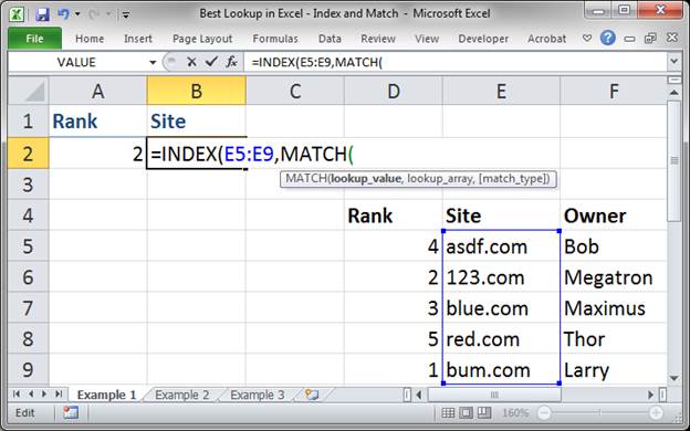
- Type a comma to go to the next argument. This argument tells the INDEX function which row to get data from, and we use the MATCH function to figure that out. Type MATCH(
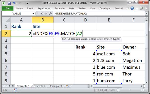
- Select the cell that contains the value that will be used to search through the table, the lookup_value cell.
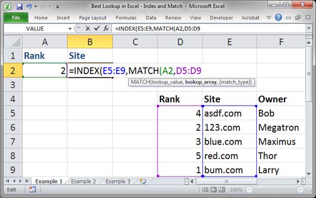
- Type a comma and then select the column of data through which we will search, in this case, the Rank column.
- Type a comma and then type 0 (zero) to make sure the lookup only returns an exact match.
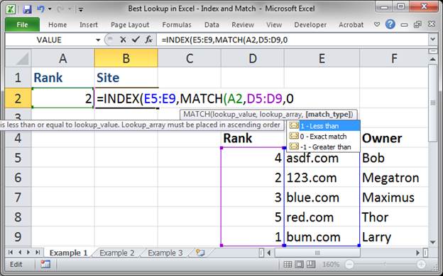
Then put two closing parentheses after the zero.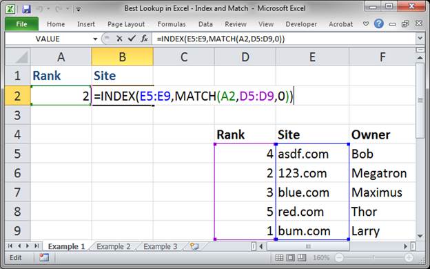
- Hit enter and that's it!
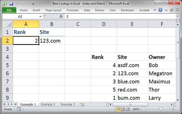
Now, if you don't already have a value in cell A2, the lookup will return a #N/A error.
Type a search value into cell A2 and we get this:
The final formula that we entered is this:
=INDEX(E5:E9,MATCH(A2,D5:D9,0))
To get this to work for you, change 3 things:
E5:E9 is the range from which you want to return values, where you want the lookup function to get the values that it displays to you.
D5:D9 is the range that you use to search through the table, using the lookup_value.
A2 is the cell that contains the lookup_value that you use to search through the table/column/range.
To make this work, the two ranges that you use must be exactly the same size. It's best if they come from the same data set or table.
Create a Right-to-Left Lookup Using INDEX and MATCH
This is the real beauty of this type of lookup. We can return a value from ANYWHERE in the table!!! With a Vlookup, we can only return a value that is to the right of the lookup column.
If you read the first example above, this one is very similar.
In the example below, we want to search the "Site" column and return a value from the "Rank" column.
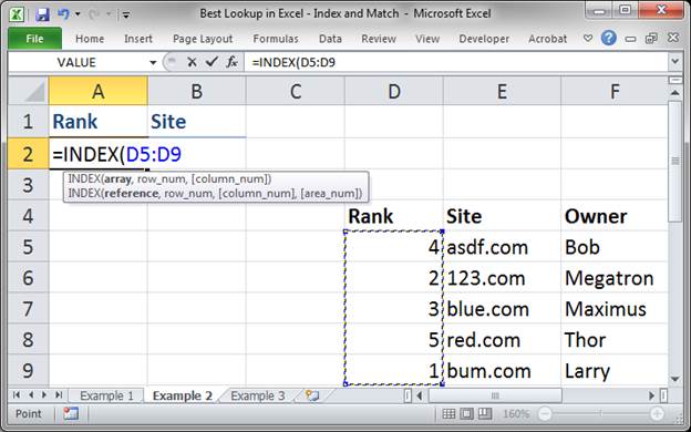
- Type =INDEX(
- Select the column of data that has the values that you want to return, the Rank column in this case.
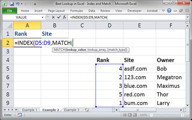
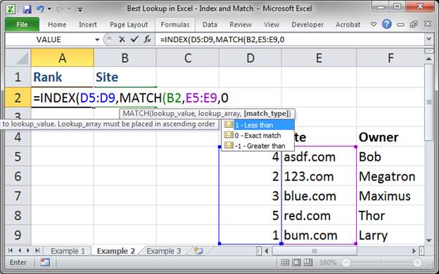
- Type a comma to move to the next argument. This argument tells the INDEX function which row to get data from, and we use the MATCH function to figure that out. Type MATCH(
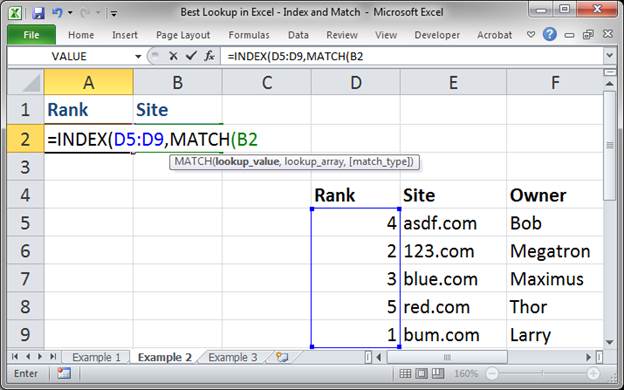
- Select the cell that will contain the value used to search through the table. In this case we want to use cell B2, which is covered by the formula at this moment, so we can just type it in by hand.
- Type a comma to move to the next argument and then select the column of data that contains the values that we will search through.
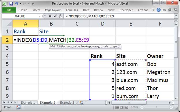
- Type a comma to move to the last argument. Type a 0 (zero) to return only exact matches in the search.
Input two parentheses to close the functions.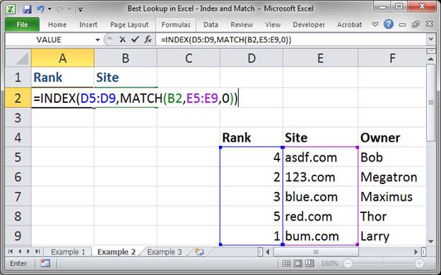
- Hit enter and that's it!
Now, if you don't already have a value in cell B2, the lookup_value cell, the lookup will return a #N/A error.
Input a search value into cell B2, in this case a site name, and we get a result like this:
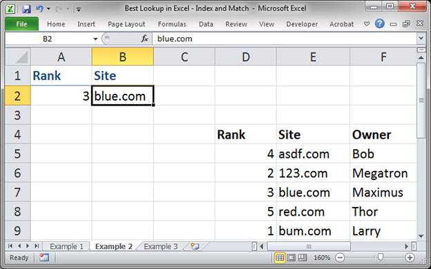
What happened here is that we performed a lookup that searched through the Site column for blue.com and returned a number from the Rank column, 3, which is located to the left of the Site column.
Now you know how to perform a right-to-left lookup in Excel!
Here is the final formula that we created:
=INDEX(D5:D9,MATCH(B2,E5:E9,0))
To get this to work for you, change 3 things:
D5:D9 is the range from which you want to return values, where you want the lookup function to get the values that it displays to you.
E5:E9 is the range that you use to search through the table, using the lookup_value.
B2 is the cell that contains the lookup_value that you use to search through the table/column/range.
As you can see, it does not matter if the column that returns the values is to the left or right of the lookup range. The only IMPORTANT thing is that the columns have to be the same size, and it helps if they are also in the same table. As a rule of thumb, make sure both columns you input into this formula are from the same data set/table; this will make things much easier for you.
Create a Two-Way Lookup Using INDEX and MATCH
This allows you to search up and down and also left and right at the same time using a single formula.
This is a confusing formula to use at first, so I will go step-by-step to tell you how to input it and then make it work for your code. This follows the same principal as the above examples; however, we need to add an additional set of steps.
In this example I will use two values to perform the lookup, one to search for a specific Site and one to return data for a specific year for that Site.
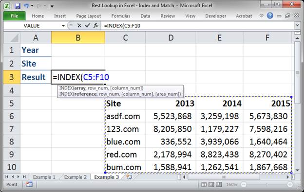
- Type =INDEX( into a cell
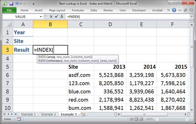
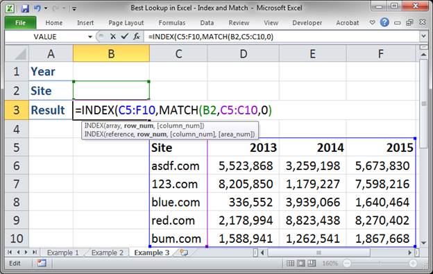
- Select the range of cells that contain the values that we want to display or return using this lookup function. We could select just the values that we want to return or the entire data table. To keep it simple and versatile, I will select the entire data table, including the header row.
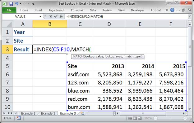
- Type a comma to move to the next argument. This argument tells the INDEX function which row to get data from and we use the MATCH function to figure that out. Type MATCH(
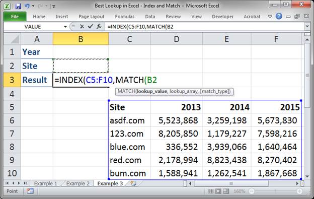
- Since this MATCH function will return the row that we need, we need to think about what we want to use to find the correct row. We will use the Site to do this. Here, select a cell that you want to use to enter the Site into so this formula can search by that. Here, we'll select cell B2.
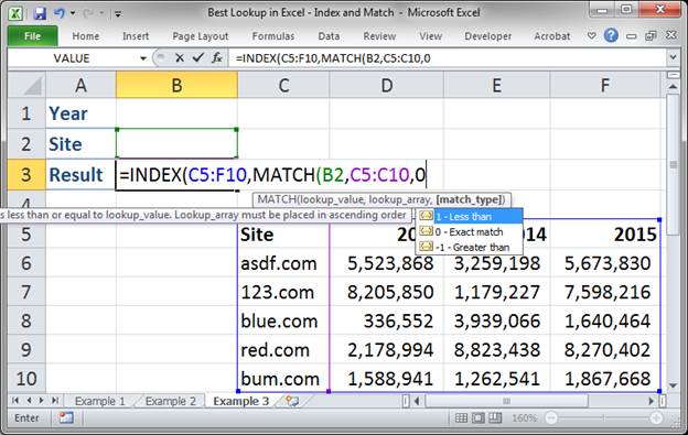
- Type a comma. And, now, since we are searching through the Site column for this MATCH function, select the Site column.

Since I included the header in the first argument for the INDEX function (Step 2), I must also include the header when selecting the Site column here. - Type a comma. Input 0 (zero) to make sure the function searches for an exact match only.
- Input ONE closing parenthesis.
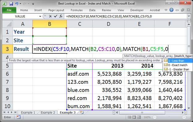
- Now, we need to move to the Column argument for the INDEX function and input another MATCH function. This is what allows us to also search by columns in this formula.
Type a comma to move to the next argument for the INDEX function and then type MATCH(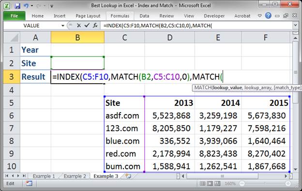
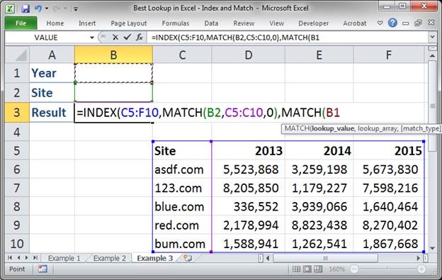
- Select the cell that will contain the value we use to search through the columns.
- Type a comma to move to the next argument. Select the row of the table that contains year numbers since that is what we will use to figure out which column we want to use to return data.
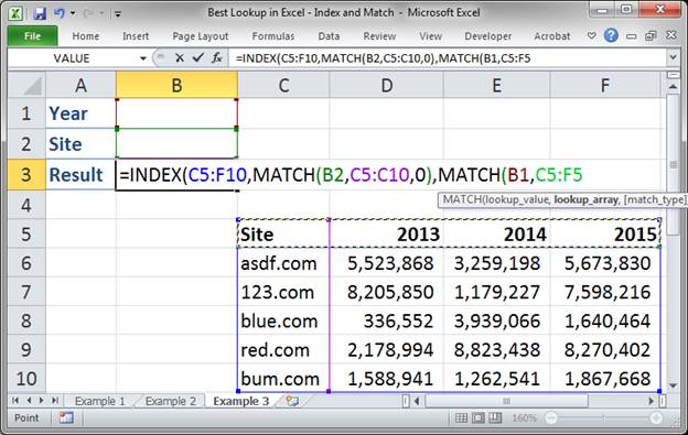
Note that I included the entire header, including where it says Site. That is not a problem and is actually required since, in Step 2, I also included the Site column. If I did not include the Site column in Step 2, I should not include it here. - Type a comma. Then, type a 0 (zero) to make sure an exact match search is performed.
- Type two closing parenthesis.
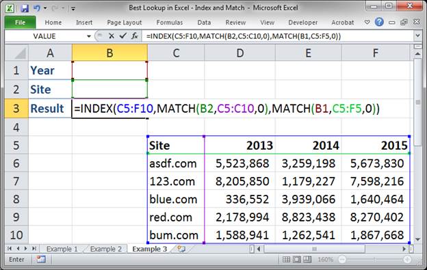
- Hit Enter and that's it! Finally!
Now, at first, you will see an error message like this: #N/A and that is just because there is no value for Year or Site yet.
Once we fill out the values for Year and Site, it looks like this:
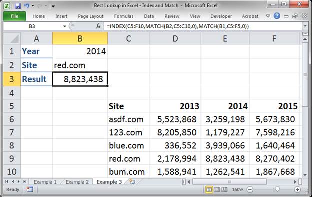
You can see that the search was performed to find red.com and then to find the data for year 2014.
Here is the final formula that was used:
=INDEX(C5:F10,MATCH(B2,C5:C10,0),MATCH(B1,C5:F5,0))
Follow the instructions above carefully the first few times you make this formula so you can get a feel for it. Once you do that, there are only a few things that you need to change to make it work with any data set.
To get this to work for you, change 5 things:
C5:F10 is the table that contains the data set.
B2 is the cell that will contain the value you will use to search through the rows to find the correct row.
C5:C10 is the range that you use the value in cell B2 to search through in order to find a match to know from which row to return data.
B1 is the cell that contains the value that you use to determine from which column to return data.
C5:F5 is the range that you use the value in cell B1 to search through in order to find a match and know from which column to return data.
Notes
The INDEX MATCH lookup function is very powerful and allows you to do things that you simply can't do with a Vlookup or Hlookup function. The problem is that it is quite complex and confusing. But, trust me, once you get started using this method and become comfortable using it in different ways, you will consider this a miracle function that saves you hours of time and many headaches.
Make sure to download the sample file attached to this tutorial so that you can follow along and get a better grasp of how to use this formula.
Question? Ask it in our Excel Forum
Excel VBA Course - From Beginner to Expert
200+ Video Lessons 50+ Hours of Instruction 200+ Excel Guides
Become a master of VBA and Macros in Excel and learn how to automate all of your tasks in Excel with this online course. (No VBA experience required.)
Subscribe for Weekly Tutorials
BONUS: subscribe now to download our Top Tutorials Ebook!
Excel VBA Course - From Beginner to Expert
200+ Video Lessons
50+ Hours of Video
200+ Excel Guides
Become a master of VBA and Macros in Excel and learn how to automate all of your tasks in Excel with this online course. (No VBA experience required.)