Apply Conditional Formatting to Multiple Cells with a Single Formula

How to use a single formula to apply conditional formatting to multiple cells at once in Excel.

This saves you the time of changing a formula for each cell and then individually adding the conditional formatting to it.

Steps

Create the formula that you want to use within the worksheet so that you can make sure that it is working.

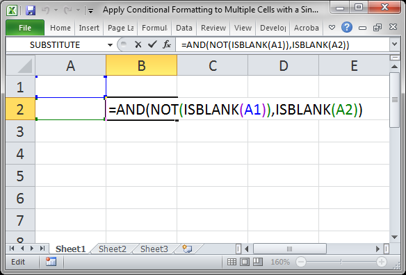
Remember that a formula for conditional formatting must evaluate to TRUE or FALSE. Our formula does just that:

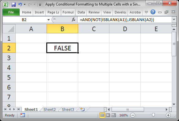
Now, figure out if the formula will apply to multiple columns, or rows, or both. In this example, I want to copy the formula down column A so that each cell will be highlighted if cell A1 has a value in it but the current cell is empty. To address this, the cell references need to be made absolute or relative.

I need A1 to remain the same when the formula is copied so I need to change that to $A$1 which makes that cell reference absolute; it will not change when the formula is copied.

I need A2 to change when the cell is copied down the column so I could leave it as it is or change it to $A2 putting the dollar sign only in front of the column but not the row; this means the column will never change but the row will change when it is copied down.

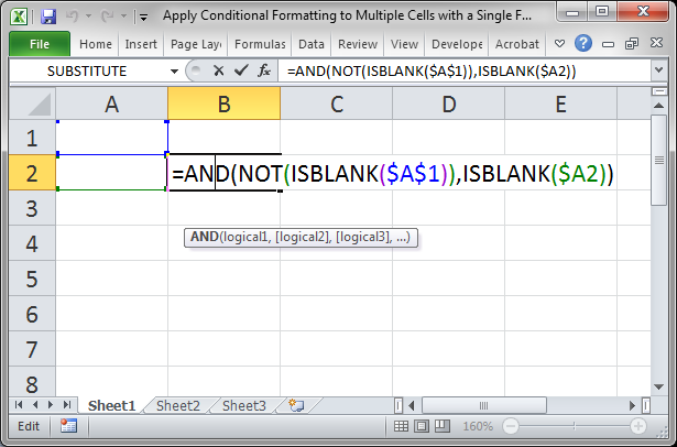
For more on cell references, view our tutorial on absolute and relative cell references in Excel.

Once your formula is ready to go, you can now add the conditional formatting:

1. Select all of the cells for which you want to apply the formatting:
   
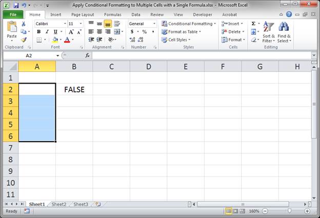
2. Go to the Home tab and click Conditional Formatting > New Rule...
   
   
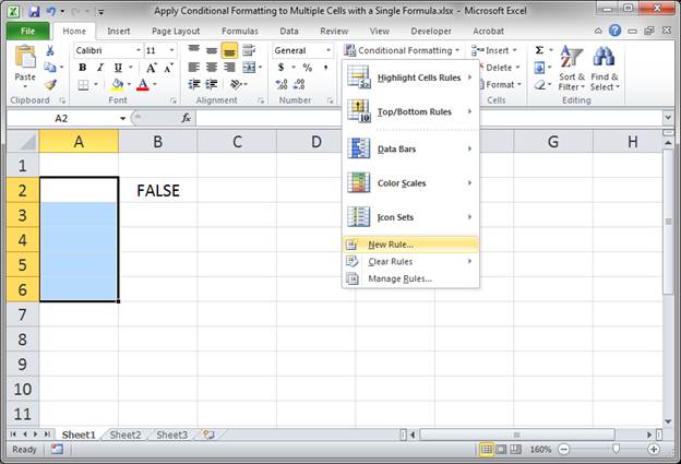
3. Select Use a formula to determine which cells to format and paste the formula that you just created.
   
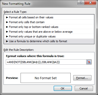
4. Click the Format button and choose the desired look for the cells.
   
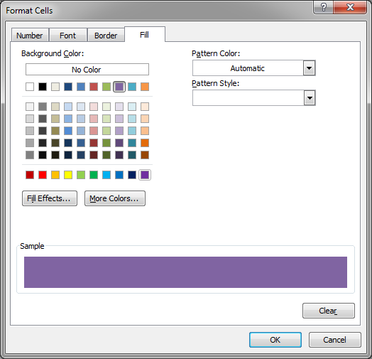
   Hit OK for the Format window and then OK again for the next window and you should be good to go.
5. Test it out:
   

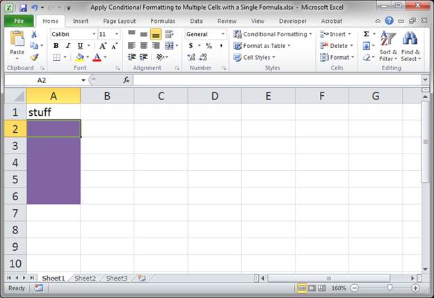
Alternatively, you could have applied the conditional formatting just to cell A2 and then selected that cell and dragged the quick-fill-handle down to copy the conditional formatting to the other cells; that works nice when there is no content currently in the destination cells.

Notes

The most important thing here is to get the formula right before you try to apply the conditional formatting. Often times, people mess-up the absolute/relative cell references in the formula and this is why the conditional formatting doesn't behave as desired.

Make sure to download the attached file for this tutorial so you can work with this example in Excel.