Formula to Get the Last Value from a List in Excel

Formulas that you can use to get the value of the last non-empty cell in a range in Excel. These examples include simple formulas and more robust complex formulas that allow you to do things like account for errors, blank cells, get the last number, and return values that begin with certain text.

Sections:

Simple Formula to Get Value of Last Non-Empty Cell

Most Robust Formula to Get Value of Last Non-Empty Cell

Notes

Simple Formula to Get Value of Last Non-Empty Cell

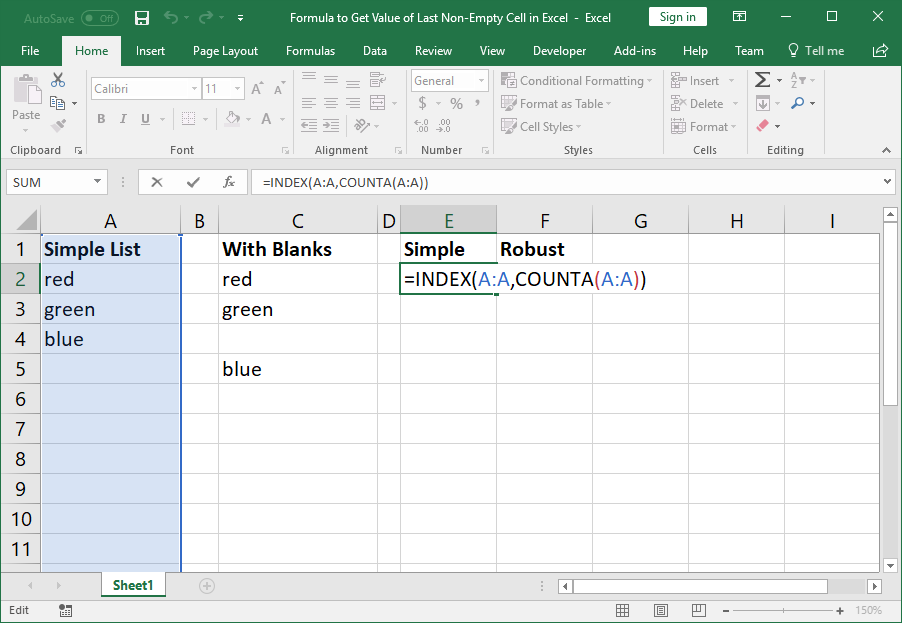
For this to work, there must be no blanks in the list of values; if that's an issue for you, look to the next section for the robust version of the formula.

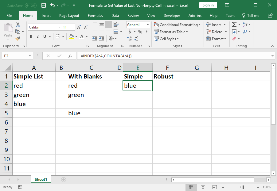
=INDEX(A:A,COUNTA(A:A))

A:A represents column A, the column with the data. If you have a large data set, just use the first column of data as the reference.

Result:

When to Use This Formula

When there are no blank cells or rows in the data set. This formula would not work correctly if we used it for the data in Column C.

The reason that this formula is included is because it is easier to remember and input and it will work for many data sets, especially data sets that are imported and that will never have blanks.

However, the next formula is more robust and will work even when your data set isn't perfect and contains blanks.

Most Robust Formula to Get Value of Last Non-Empty Cell

This works even if there are empty rows in the data set; however, it can be a bit confusing.

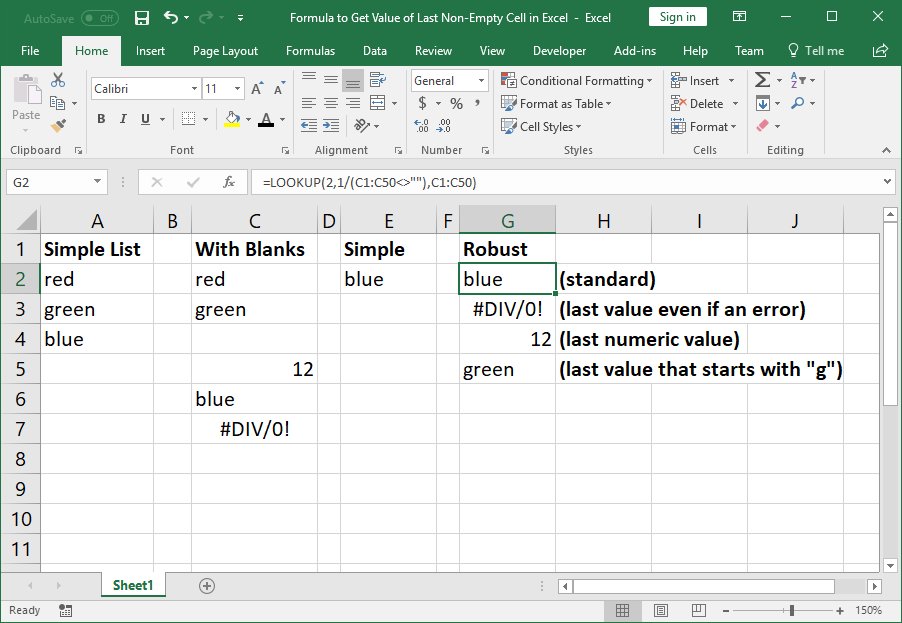
=LOOKUP(2,1/(C1:C50<>""),C1:C50)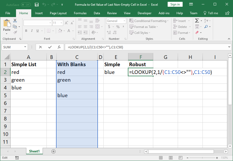

This formula gets the value of the last non-empty cell from column C within the range of C1 to C50.

C1:C50 is the range in which your data set will appear. You can only use one column for reference in this formula, so do not include the reference of the entire range for a large table, just a single column. Also, both range references in the formula must be exactly the same.

When using this for your data, do not include the entire column reference like C:C because it will make the formula run slowly as it will have to cycle through every cell in the column, regardless of it it contains data or not; simply use a range that is large enough to always encompass your data set.

Formula Explanation

This is a confusing formula and, honestly, you don't need to read this section, just copy/paste the above formula to your worksheet, change the range references and use the result.

1. C1:C50<>"" checks the range C1:C50 for empty cell or not and returns a list of TRUE/FALSE values for the cells in range C1:C50. TRUE if the cell is not empty and FALSE if it is.
2. 1/ does the task of dividing 1 by the TRUE/FALSE values from step 1. TRUE is the same as 1 and FALSE is the same as 0, so it returns either 1 or an error, #DIV/0!, which is caused because you can't divide by zero. The entire list of 1's and errors is kept in the LOOKUP function, where it is evaluated in step 3.
3. 2 is the value that the LOOKUP function tries to find in the list of values created in step 2. Since it can't find the number 2, it looks for the next highest value, which is 1, and it looks for this value starting from the end of the list and going to the beginning of this list. It stops when it hits the first result, which will be the last cell in the range that has a value in it, which was turned into a 1 in step 2.
4. C1:C50 is the last argument of the LOOKUP function and it causes the value of the cell to be returned instead of the value gotten from step 2.

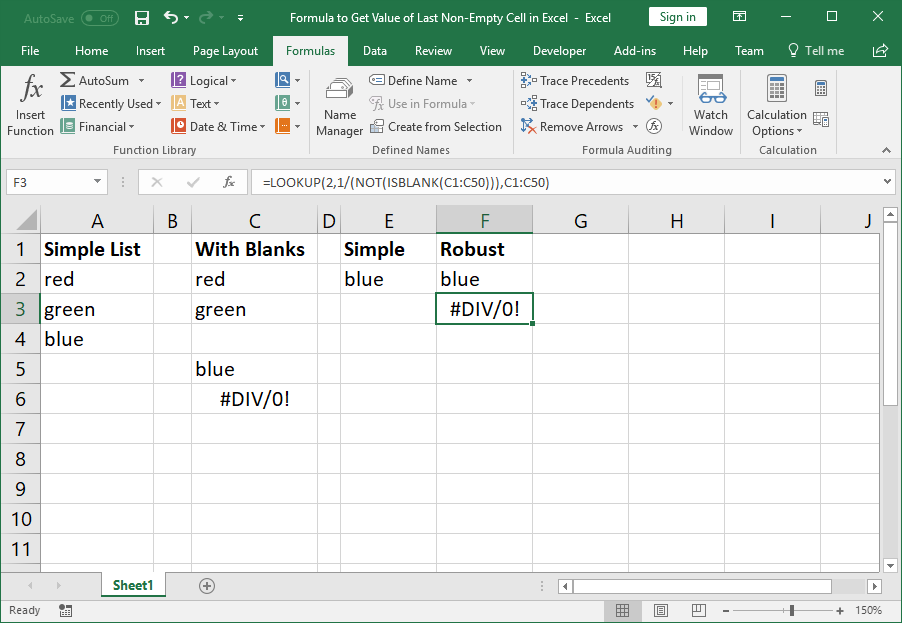
Account for Errors

If the last cell in the range outputs an error and you want that to appear when it happens, use this version of the above formula:

=LOOKUP(2,1/(NOT(ISBLANK(C1:C50))),C1:C50)

C1:C50<>"" was replaced with NOT(ISBLANK(C1:C50))

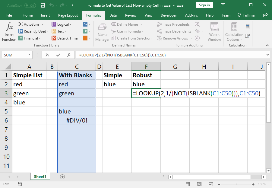
Result:

Last Numeric Value

Get the last value in the list that is a number.

=LOOKUP(2,1/(ISNUMBER(C1:C50)),C1:C50)

C1:C50<>"" was replaced with ISNUMBER(C1:C50)

This checks if the value in the cell is a number or not and uses that to create the TRUE/FALSE values.

Last Value that Begins with Some Value

=LOOKUP(2,1/(LEFT(C1:C50,1)="g"),C1:C50)

C1:C50<>"" was replaced with LEFT(C1:C50,1)="g"

This checks if the value in the cell starts with the letter g or not and uses that to create the TRUE/FALSE values.

Make Your Own

As you can see, you can use the LOOKUP function to create a rather robust series of tests to get the last value from a list so long as that value meets certain criteria.

In the above examples, we used the ISNUMBER, LEFT, NOT, & ISBLANK functions to show you some of the variations that you can make, but you are not limited to these; play around with the function and see what kinds of results you can get, it can make your data reporting a lot more useful.

Notes

These formulas are not array formulas!

You can use the entire column range reference if you want, but it can really slow down the performance of your spreadsheet, so be careful with that; usually, it's best to use a range that is sufficiently large enough to encompass the entirety of your data, now and into the future, but not the entire column.

Make sure to download the attached spreadsheet so you can view these examples in Excel.