CHOOSE Function in Excel
Return a value from a list of values. This is like a mini-lookup function that contains all of the values within itself.
The CHOOSE() function allows you to enter a list of data into it and retrieve the desired value based on its position within that list.
Sections:
Syntax
=CHOOSE(index_num, value1, [value2],)
| Argument | Description |
|---|---|
| Index_num | Says which value in the list of values will be output. The list of values is made up of the value arguments that follow this argument. There can be up to 254 value arguments and so the index_num can be from 1 to 254. |
| Value1 | This is the first value from which the Index_num argument can select. If the index_num argument is 1, then this value will be selected and output by the CHOOSE function. This can be a cell reference, number, or text (text must be surrounded by quotation marks). |
| [Value2] | Any value after Value1 is optional. You can have up to 254 value arguments, which is the same as having a list of 254 values that can be returned by the CHOOSE function. |
[] means the argument is optional.
The CHOOSE function acts like a self-contained array variable where you use the Index_num argument to get the desired value back from the function.
In other words, the CHOOSE function holds a list of values and then returns one of those values based on the number in the Index_num argument.
This may sound a bit confusing so let's get to some examples.
Example - Basic
Let's start off with a very basic example so you can see how it works.
=CHOOSE(1,"hi","bye")
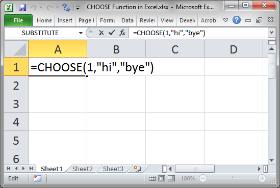
Index_num is 1, which means that the value from the first value argument (Value1) will be returned by the function.
Value1 is the text value hi and since it is text it must be surrounded with quotation marks. Numbers do not need quotation marks around them.
Value2 is another text value. Remember that Value2 is optional but you can have up to 254 values, value arguments, in this function. If Index_num was 2, then this value would be output.
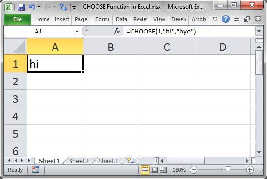
The index_num is telling the function to return the first value, which is "hi" and so the result is this:
Example - More Useful
This example is slightly more complex, but it will give you a better understanding of how this function can be really helpful.
Let's create a formula that will output the day of the week based on the date. Using CHOOSE, I can use custom names for the days.
=CHOOSE(WEEKDAY(A3),"Sunday Funday", "Sad Monday", "Boring Tuesday", "Hump-Day", "Thursday Drink Special", "Friday Finally", "Saturday YEAH")
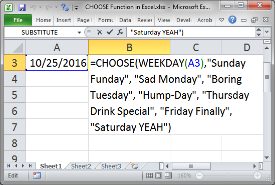
This gets the day of the week from the date in cell A3 and then returns the name for that day based on the list of names that I entered for the Value arguments. I used custom names for the day just because it's more fun.
Index_num contains the function WEEKDAY(A3) which returns the day of the week in a number format from 1 to 7. This allows us to input 7 values for the days of the week and then get the correct result.
Value there are 7 Value arguments, one for each day of the week. Since the WEEKDAY function returns 1 to 7 depending on the day of the week, I just need to make sure that I input the days of the week in the correct order.
Here is the result:
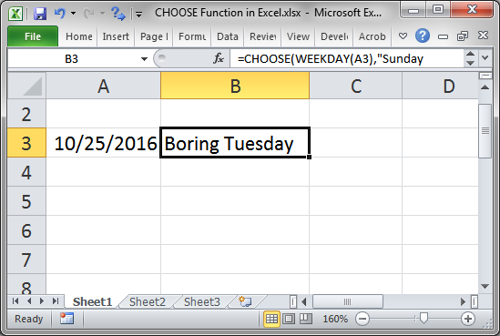
The most important thing is to make sure that the number for the Index_num argument corresponds to one of the Value arguments.
Notes
The CHOOSE function seems rather boring at first and not very helpful and, to be honest, you probably won't use it too much. But, when the correct situation arises, this will save you a lot of time and effort over other solutions in Excel, many of which would require a separate table and a Vlookup, Hlookup, or Index/Match formula.
Make sure to download the sample file for this tutorial to work with the above examples in Excel.
Question? Ask it in our Excel Forum
Excel VBA Course - From Beginner to Expert
200+ Video Lessons 50+ Hours of Instruction 200+ Excel Guides
Become a master of VBA and Macros in Excel and learn how to automate all of your tasks in Excel with this online course. (No VBA experience required.)
Tutorial: In this tutorial I will cover the basic concepts of Formulas and Functions in Excel. A for...
Tutorial: How to create a custom worksheet function in Excel. These are called User Defined Function...
Macro: Determine if a cell in Excel contains a formula or function with this UDF (user defined fu...
Tutorial: Full explanation of the Vlookup function in Excel, what it is, how to use it, and when yo...
Tutorial: In this tutorial I am going to show you how to easily input complex Functions in Excel. To...
Tutorial: The OFFSET function in Excel returns a cell or range reference that is a specified number...
Subscribe for Weekly Tutorials
BONUS: subscribe now to download our Top Tutorials Ebook!
Excel VBA Course - From Beginner to Expert
200+ Video Lessons
50+ Hours of Video
200+ Excel Guides
Become a master of VBA and Macros in Excel and learn how to automate all of your tasks in Excel with this online course. (No VBA experience required.)