MAX and MIN Values from a Filtered List in Excel

How to get the MAX and MIN values from a filtered data set. This method returns the value from only the visible rows after data has been filtered.

To do this, we use the SUBTOTAL() function.

Sections:

Syntax

Example - Filtered Data

Example - Exclude Manually Hidden Rows

Notes

Syntax

MAX

=SUBTOTAL(4, range)

4 tells the function to return the max value.

range is the range from which you get the max.

MIN

=SUBTOTAL(5, range)

5 tells the function to return the min value.

range is the range from which you get the value.

Example - Filtered Data

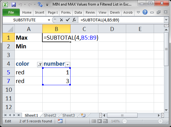
=SUBTOTAL(4,B5:B9)

This gets the max value from the range in a filtered data set. B5:B9 is the range.

Use 4 or 5 for the first argument to get the MAX or MIN value. Other than that, the syntax is exactly the same.

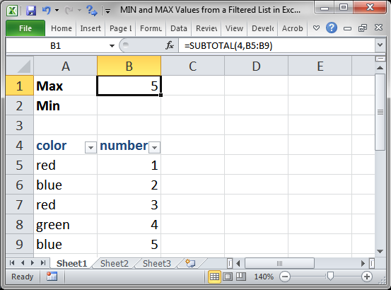
Result:

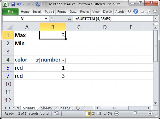
This works if the data is filtered or unfiltered.

MIN or MAX

Change the first argument to return a min or a max.

4 means to return the MAX.

=SUBTOTAL(4,B5:B9)

5 means to return the MIN.

=SUBTOTAL(5,B5:B9)

Example - Exclude Manually Hidden Rows

The above example will not work on data that is manually hidden (right-click a row and click Hide).

To make the SUBTOTAL function also ignore manually hidden cells, we must put 10 in front of the number for each argument.

Max

=SUBTOTAL(104,B5:B9)

Min

=SUBTOTAL(105,B5:B9)

104 replaced the 4 to return the Max.

105 replaced the 5 to return the Min.

Nothing else changed.

Notes

This is a great function to use to return the Min and Max value from a list of data that you are analyzing. In fact, even if you are not performing a filter right now, but you think you might in the future, it can be a good idea to use the SUBTOTAL function instead of the MIN and MAX functions just so that you can later filter the data and still have accurate results.

The SUBTOTAL function allows you to apply a number of regular functions to filtered data, for a full list and explanation, view our tutorial on the SUBTOTAL function in Excel.

Make sure to download the file for this tutorial so you can work with the above examples in Excel.