Make Complex Formulas for Conditional Formatting in Excel

How to make complex formulas for conditional formatting rules in Excel. This will serve as a guide to help you build the formulas that you need for conditional formatting custom rules.

Sections:

Make a Formula for Conditional Formatting

Making Complex Formulas

Notes

Make a Formula for Conditional Formatting

Every formula that you use for conditional formatting must evaluate to True or False. That means that if you put that formula into a worksheet, the output would be True or False. This is the most important aspect of making conditional formulas.

Once you have a formula that you want to enter, select the desired cell and go to the Home tab > Conditional Formatting > New Rule > select Use a formula to determine which cells to format and then enter the desired formula in the input box and click the Format button to choose what the cell will look like if the formula evaluates to True.

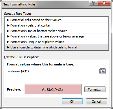
Here, I am using a simple function to see if the cell is blank or not:

=ISBLANK($A$1)

This is a simple formula and I just typed it into this window, but, for complex formulas, follow the guide in the next section.

Making Complex Formulas

Complex formulas should always be made and tested in the worksheet before you put them into a conditional formatting rule.

This is because the place where you input formulas for conditional formatting does not check the formula for errors and you cannot troubleshoot issues.

When you create the formula in the worksheet, you can visually see that the correct cells are referenced, check the output of the formula under different conditions, and basically verify that they work correctly.

Note: all formulas used for conditional formatting must evaluate to True or False.

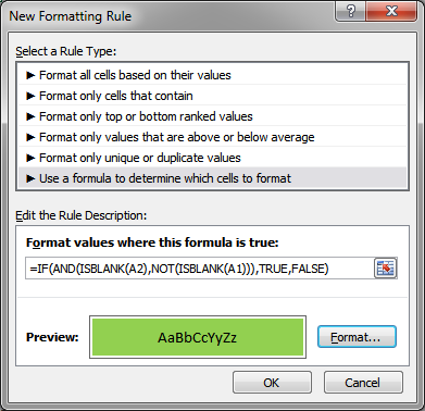
Here is our sample formula:

=IF(AND(ISBLANK(A2),NOT(ISBLANK(A1))),TRUE,FALSE)

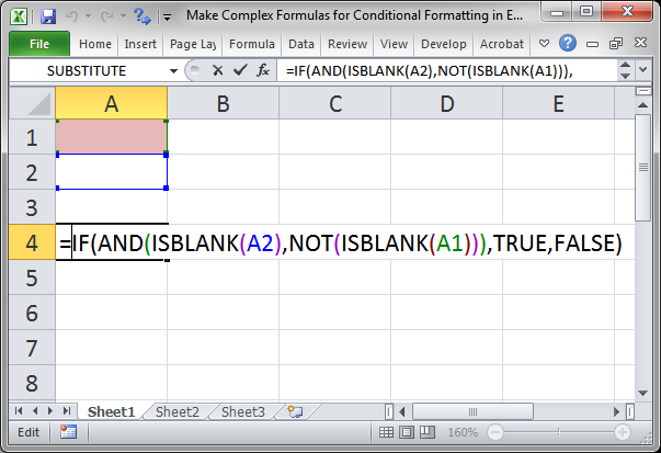
Though it's not terribly complex, you can see that the syntax is highlighted and the cells involved in the formula are also highlighted and it is generally easy to read and understand.

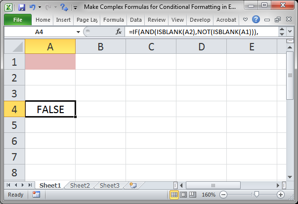
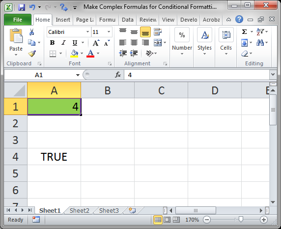
Also, when I hit Enter, you can see the output and ensure that it is correct:

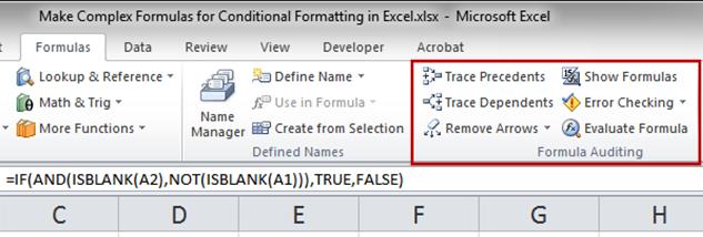
While the formula is here in the worksheet I can run formula auditing on it to ensure that it is working exactly the way that I want it to work.

Go to the Formulas tab and the Formula Auditing section to see these tools:

Insert Formula into Conditional Formatting

Once you have a tested and working formula, put it into the Conditional Formatting feature.

Select the desired cell and then go to the Home tab > Conditional Formatting > New Rule > select Use a formula to determine which cells to format and then paste the formula into the input box and click the Format button to choose what the cell will look like when the formula evaluates to True.

Hit OK and you will see the result:

Notes

Do not hit any of the arrow keys to move the cursor within the formula input area for Conditional Formatting; doing this will cause cell references to be input into the formula and it is a real pain to remove them. Follow the instructions above and you will avoid all major issues when it comes to using formulas with Conditional Formatting in Excel.

I left the formula for the last example in the sample file so it is easier for you to see but, in practice, you should remove it once you add it to Conditional Formatting.

Make sure to download the sample file for this tutorial so you can work with the above examples in Excel.